Shallow-water experiments on the sphere

This site presents MITgcm shallow-water verification experiments, including the Williamson standard test cases and free-surface initialization runs over constant and real bathymetry. Each section collects the governing equations, expected output, numerical settings, snapshots, and available result diagnostics.

Code and website by Hoda Hashemi.

Time-Step Safety Check (CFL)

This section checks whether each submitted model time step is small enough for the resolved velocities and grid spacing.

Grid1440 x 720
Min dx60.65 m
dy27.80 km
Warn CFL0.5

Equations

The advective audit uses the local spherical-polar metrics from the 0.25 degree grid:

\[C_{adv}=\Delta t\left(\frac{|u|}{\Delta x}+\frac{|v|}{\Delta y}\right)\]
\[\Delta x=a\cos\phi\,\Delta\lambda,\quad \Delta y=a\Delta\phi\]
\[C_g=\frac{\sqrt{gH}\,\Delta t}{\Delta x}\]

The polar row dominates the metric audit: center-cell dx_min=60.65 m, while dy=27798.73 m. The gravity-wave CFL is shown as an explicit-wave diagnostic only because every active data file has implicitFreeSurface=.TRUE..

How deltaT Was Chosen

The template input/data files provide the grid and default schedule, but the submitted Slurm files are the source of truth for vortexSphere runs. Each job exports DELTA_T, computes nTimeSteps=round(TOTAL_SECONDS/DELTA_T), copies the input directory, then rewrites the run-local data file. The table keeps template, job, and archived-run deltaT separate.

TC1 has two entries here: the vortexSphere TC1 rows use the submitted lat-lon jobs, while TC1 cubed rows are MITgcm advect_cs runs and keep the tutorial timestep deltaT=2700 s. The cubed CFL values come from MITgcm monitor output.

The Run dir column is the exact archived directory whose run-local data file was used for the timestep row.

The mild tilts use 10 s, the verified TC2 high tilts use 1.0 s and 0.5 s, the standard zonal cases use 60 s, and TC6 uses 30 s.

Decision

No completed run exceeds advective CFL 1.0. In the verified TC2 suite, alpha=0.05 and alpha=1.52 are above the conservative 0.5 saved-output margin, so use deltaT<=8.30 s and deltaT<=0.69 s, respectively, if that extra margin is required. TC2 alpha=1.57 uses the completed 0.5 s rotated-Coriolis run and remains below the 0.5 margin. TC5 is now a completed CS32 rerun: final saved state fields are finite through day 15, and the mountain is verified as static bathymetry rather than an eta bump. TC6 is the completed Rossby-Haurwitz run_standard row at deltaT=30 s for 40320 steps. TC7 uses cubed-sphere compact initial fields for the submitted three-date suite.

n/a means the audit could not read a finite CFL source for that column: missing archived U/V fields, unavailable initial-velocity hook, or a cubed-sphere row where the spherical-polar gravity-wave metric is not used. TC4 now includes both run_u0_20 and completed run_u0_40 output.
Compact CFL Table

CaseRunRun dirdt(s)n stepstotal(s)daysmax CFLStatus/action
TC1alpha=0run_alpha_060.017280103680012.00.083OK
TC1alpha=0.05run_alpha_0.0510.0103680103680012.00.332OK
TC1alpha=1.52run_alpha_1.520.751382400103680012.00.490OK
TC1alpha=1.57run_alpha_1.570.751382400103680012.00.477OK
TC2alpha=0run_alpha_0_latlon60.017280103680012.00.083OK
TC2alpha=0.05run_alpha_0.05_latlon_rotcori_12day10.0103680103680012.00.603OK<1; 0.5 margin dt<=8.30 s
TC2alpha=1.52run_alpha_1.52_latlon_rotcori_12day1.001036800103680012.00.728OK<1; 0.5 margin dt<=0.69 s
TC2alpha=1.57run_alpha_1.57_latlon_rotcori_12day_dt0p50.502073600103680012.00.377OK
TC3alpha=0run_alpha_0_latlon_5day_45rank60.072004320005.000.097OK
TC3alpha=1.0472run_alpha_1.0472_latlon_rotcori_5day_45rank0.508640004320005.000.399OK
TC4run_u0_20run_u0_2060.072004320005.000.139OK
TC4run_u0_40run_u0_4060.072004320005.000.193OK
TC5run_standard_cs32run_standard_cs3230.043200129600015.00.005OK
TC6standardrun_standard30.040320120960014.00.126OK
TC7run_c1_19781221_0000run_c1_19781221_000025.0172804320005.000.009OK
TC7run_c2_19790116_0000run_c2_19790116_000025.0172804320005.000.012OK
TC7run_c3_19790109_0000run_c3_19790109_000025.0172804320005.000.011OK
TC1 cubedadvect_cs alpha=0alpha_0/run_alpha_02700384103680012.00.768OK<1; 0.5 margin dt<=1757.71 s
TC1 cubedadvect_cs alpha=0.05alpha_0.05/run_alpha_0.052700384103680012.00.786OK<1; 0.5 margin dt<=1717.65 s
TC1 cubedadvect_cs alpha=1.52alpha_1.52/run_alpha_1.522700384103680012.00.786OK<1; 0.5 margin dt<=1717.65 s
TC1 cubedadvect_cs alpha=1.57alpha_1.57/run_alpha_1.572700384103680012.00.768OK<1; 0.5 margin dt<=1757.71 s
Check commands
cd /home/hmh85/scratch/MITgcm
/home/hmh85/scratch/MITgcm/.venv/bin/python Sandbox/Scripts/cfl_deltaT_audit.py --write-fragments

cd Sandbox/MITgcm_Williamson_TC1
/home/hmh85/scratch/MITgcm/.venv/bin/python tools/postprocess_advect_cs.py --check-only

cd Sandbox/vortexSphere_Williamson_TC1
/home/hmh85/scratch/MITgcm/.venv/bin/python tools/check_cfl_tc1.py --all

cd Sandbox/vortexSphere_Williamson_TC2
/home/hmh85/scratch/MITgcm/.venv/bin/python tools/check_cfl_tc2.py --all

cd Sandbox/vortexSphere_Williamson_TC3
/home/hmh85/scratch/MITgcm/.venv/bin/python tools/check_cfl_tc3.py --all

cd Sandbox/vortexSphere_Williamson_TC4
/home/hmh85/scratch/MITgcm/.venv/bin/python tools/check_cfl_tc4.py --all

cd Sandbox/vortexSphere_Williamson_TC5
/home/hmh85/scratch/MITgcm/.venv/bin/python tools/check_cfl_tc5.py --all

cd Sandbox/vortexSphere_Williamson_TC6
/home/hmh85/scratch/MITgcm/.venv/bin/python tools/check_cfl_tc6.py --all

Conservation and Output-Health Checks

This section checks whether each run output stayed finite and whether mass, transported quantity, energy proxy, and derived PV/enstrophy behave as expected.

FieldsEta / U / V
Health Gatefinite state
CasesTC1-TC7
EquationsRendered

What Is Computed

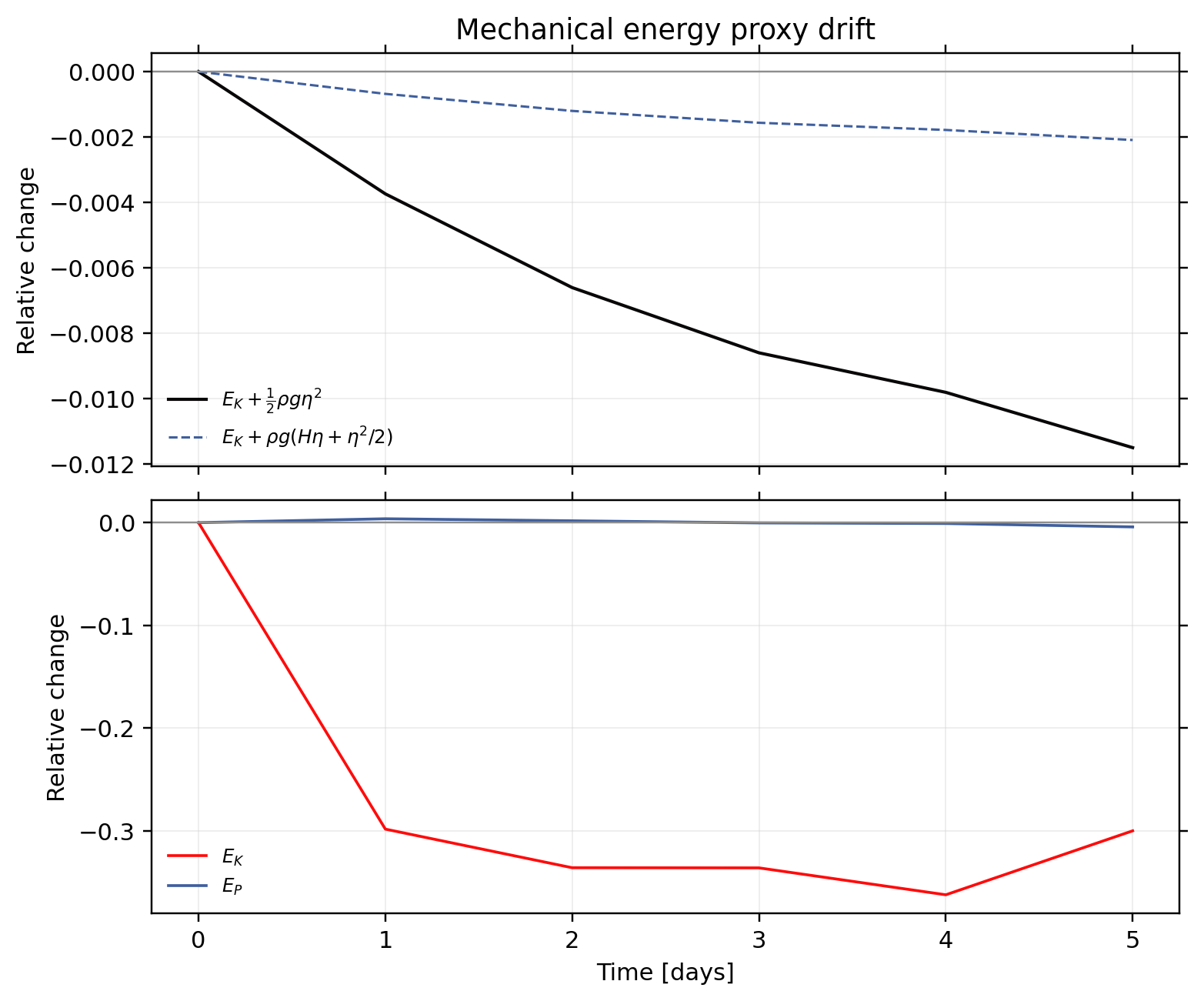
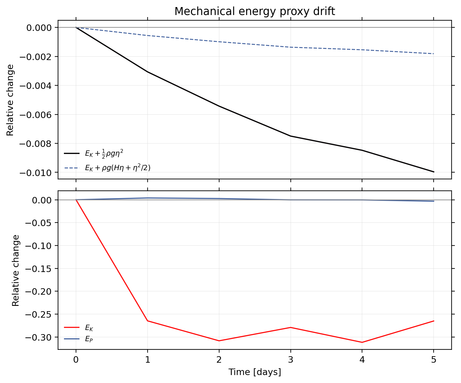
Mass and free-surface volume come from Eta/ETAN. TC1 tracer conservation uses S/SALT. The mechanical-energy proxy uses native momKE when it exists, otherwise centered U/V. Relative vorticity, PV, and potential enstrophy are derived from U/V/Eta.

Equations

Derived potential enstrophy means this quantity is reconstructed in postprocessing from saved state fields. It is not a native MITgcm output field in these runs.

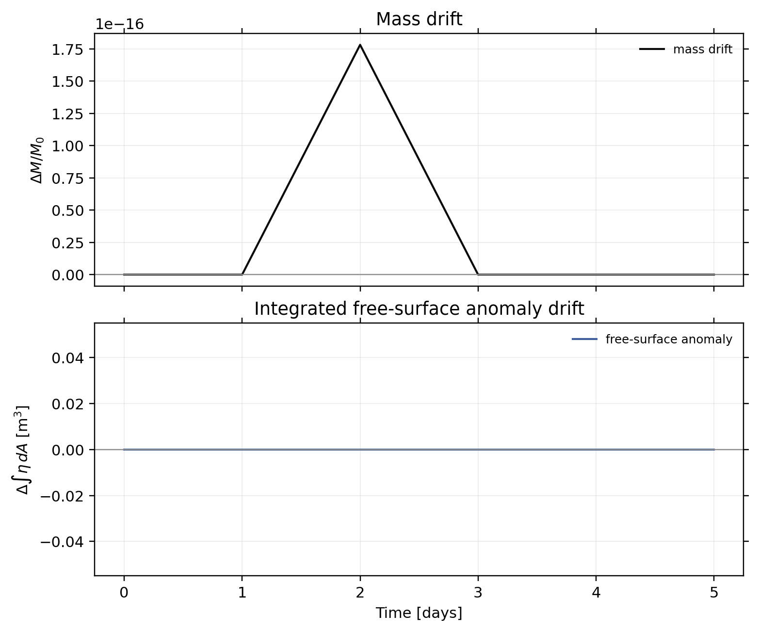
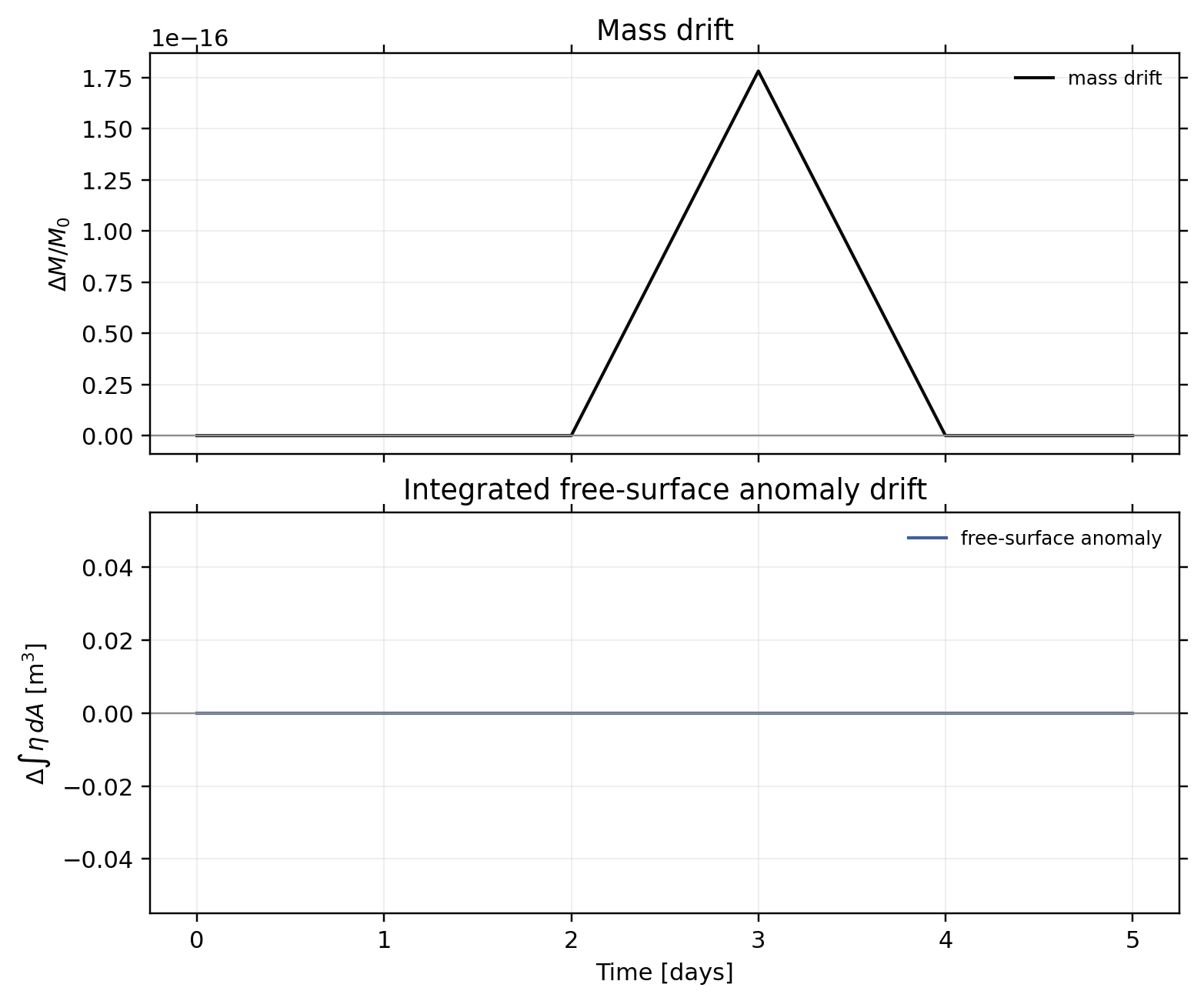
\[h = H + \eta,\qquad M = \rho_0\int_\Omega h\,dA\]
\[E_m = \rho_0\int_\Omega hK\,dA + \frac{1}{2}\rho_0 g\int_\Omega \eta^2\,dA\]
\[\zeta = \frac{1}{a\cos\theta}\left(\frac{\partial v}{\partial\lambda} - \frac{\partial(u\cos\theta)}{\partial\theta}\right)\]
\[q = \frac{\zeta + f}{h},\qquad Z = \frac{1}{2}\int_\Omega hq^2\,dA\]
\[\Delta_r X(t) = \frac{X(t)-X(0)}{|X(0)|}\]

Here K is native momKE when available, otherwise it is reconstructed as (u^2+v^2)/2. The Coriolis term f comes from fCoriC.bin when a rotated run writes it; otherwise the diagnostic uses 2*omega*sin(latitude).

Health Gate

Every saved state is checked for finite Eta, U, V, and scalar values when available. A run with all-NaN or partially non-finite later records is marked invalid even if day 0 conserves exactly.

Case Verdicts

CaseStatusMassTarget quantityEnergy proxyPV/enstrophyOutput health
Case Status Mass Target quantity Energy proxy PV/enstrophy Output health
TC1 Verified preserved to roundoff well preserved small drift small drift finite saved state fields
TC2 Verified preserved to roundoff not preserved not preserved not preserved finite saved state fields
TC3 Validated with caveat unavailable unavailable unavailable unavailable no usable run output
TC4 Verified preserved to roundoff noticeable drift noticeable drift noticeable drift finite saved state fields
TC5 Verified preserved to roundoff not preserved not preserved not preserved finite saved state fields
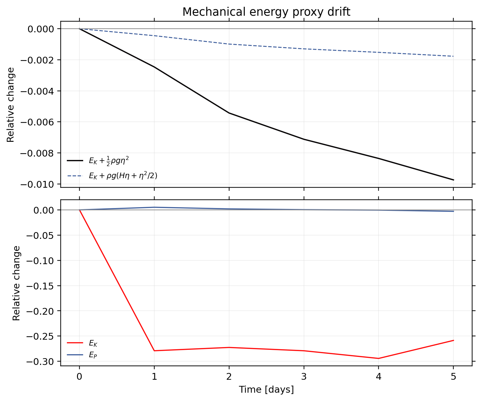
TC6 Verified preserved to roundoff noticeable drift not preserved noticeable drift finite saved state fields
TC7 Verified preserved to roundoff not a scalar test not preserved unavailable finite saved state fields
TC1 - Cosine bell passive-tracer advection Verified

Mass is preserved to roundoff (max |rel| 7.709e-16). The TC1 tracer amount is well preserved (max |rel| 6.213e-08). The energy curve is diagnostic only for this prescribed-flow tracer test.

  • alpha=0: mass preserved to roundoff; quantity preserved to roundoff; energy preserved to roundoff; PV/enstrophy preserved to roundoff
  • alpha=0.05: mass preserved to roundoff; quantity well preserved; energy small drift; PV/enstrophy well preserved
  • alpha=1.52: mass preserved to roundoff; quantity well preserved; energy small drift; PV/enstrophy small drift
  • alpha=1.57: mass preserved to roundoff; quantity well preserved; energy small drift; PV/enstrophy small drift

No plot assets are available for this case yet.

TC2 - Steady solid-body geostrophic flow Verified

Verified from the four corrected TC2 runs used on the testcase page. The saved state fields are finite through day 12 and mass is preserved to roundoff across all tilts; the steady-state error norms, not exact energy or PV conservation, are the verification gate for this balanced-flow case.

  • alpha=0: mass preserved to roundoff; quantity small drift; energy small drift; PV/enstrophy small drift
  • alpha=0.05: mass preserved to roundoff; quantity not preserved; energy noticeable drift; PV/enstrophy not preserved
  • alpha=1.52: mass preserved to roundoff; quantity not preserved; energy not preserved; PV/enstrophy not preserved
  • alpha=1.57: mass preserved to roundoff; quantity not preserved; energy not preserved; PV/enstrophy not preserved

The TC2 testcase section links the exact day-12 error norms and postprocessing assets used for verification.

TC3 - Steady compact-support zonal flow Validated with caveat

Unavailable: no usable run output found

  • No conservation output found.

No plot assets are available for this case yet.

TC4 - Forced nonlinear exact solution Verified

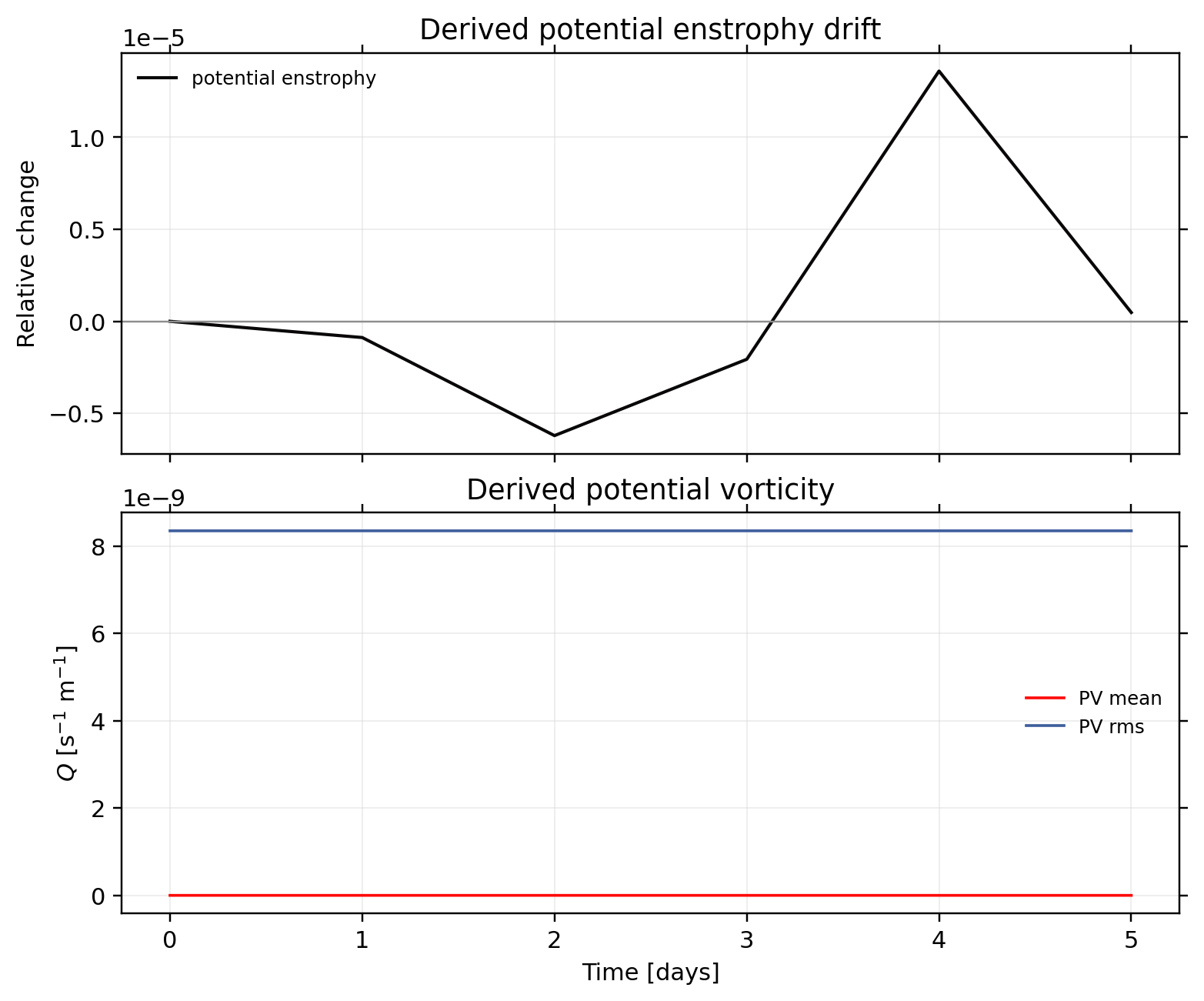
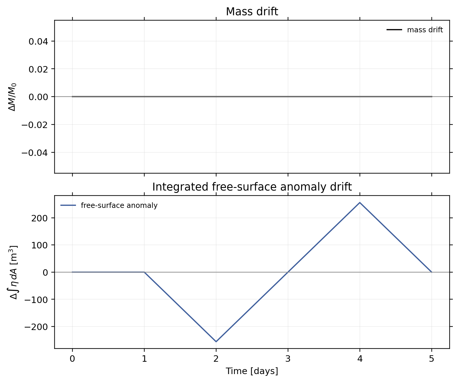
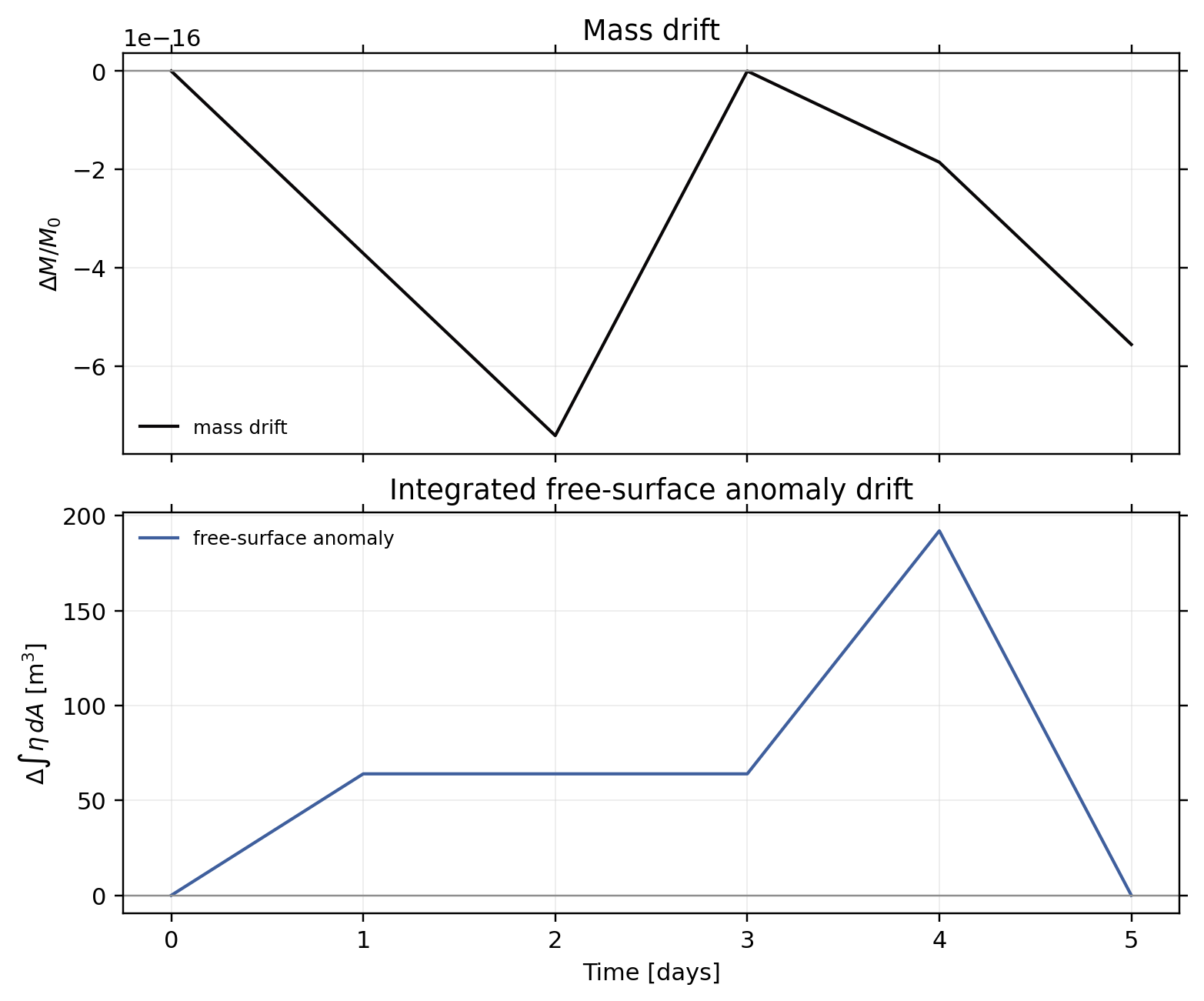
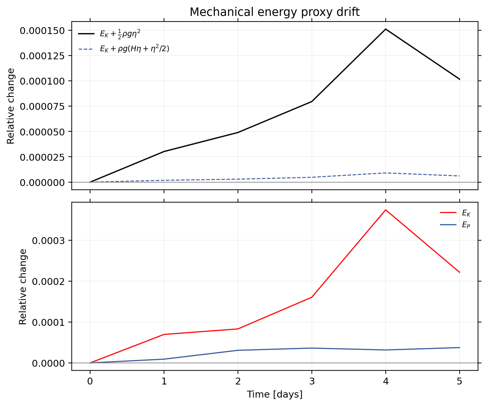
Mass is preserved to roundoff (max |rel| 7.406e-16). Because TC4 is analytically forced, the mechanical-energy and derived potential-enstrophy curves are diagnostic traces, not unforced conservation claims (energy max |rel| 1.511e-04, enstrophy max |rel| 1.360e-05). Together with the analytic path check and published snapshots, the c1 output is marked verified.

  • alpha=run_u0_40: mass preserved to roundoff; quantity noticeable drift; energy noticeable drift; PV/enstrophy noticeable drift
TC5 - Zonal flow over an isolated mountain Verified

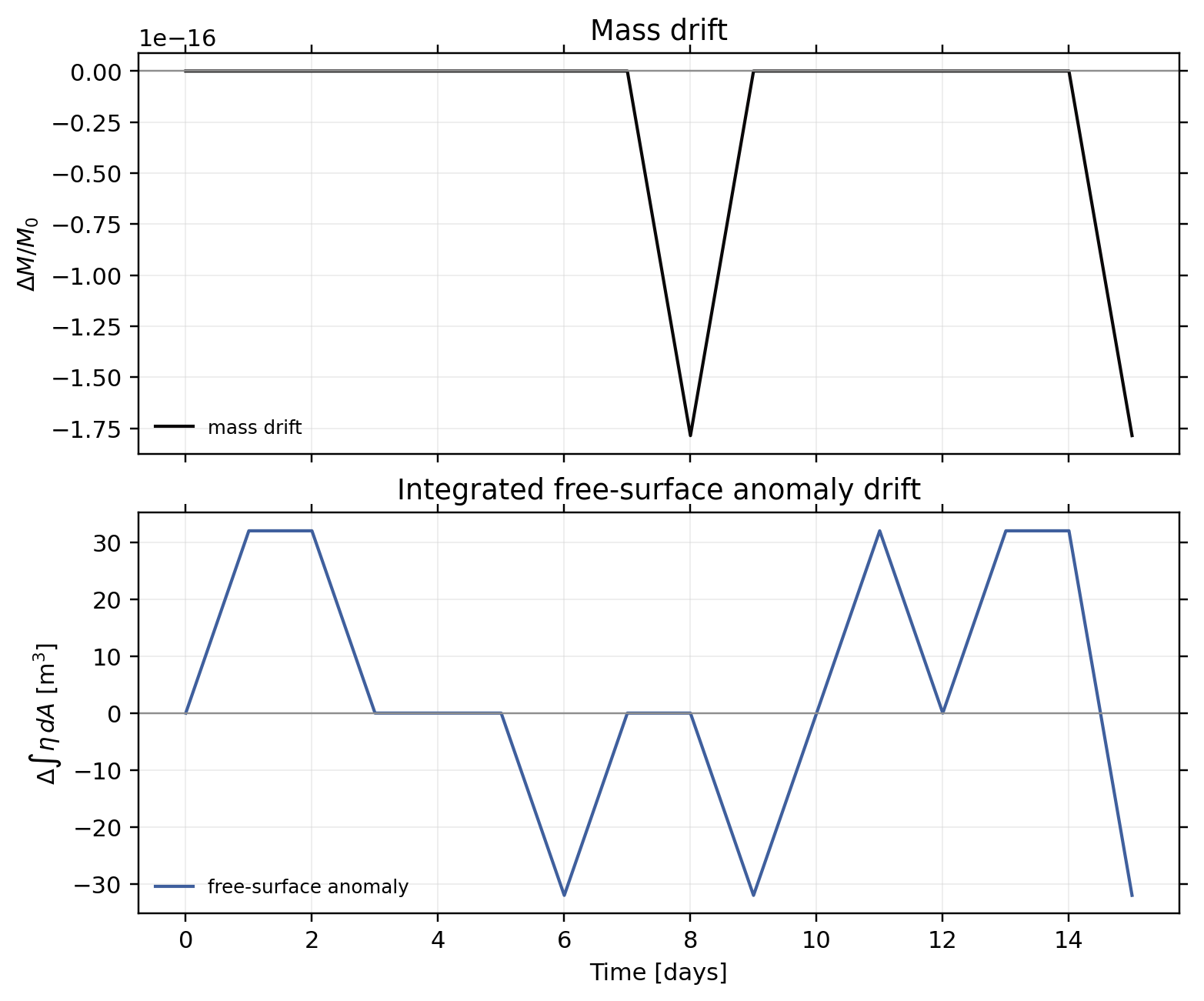
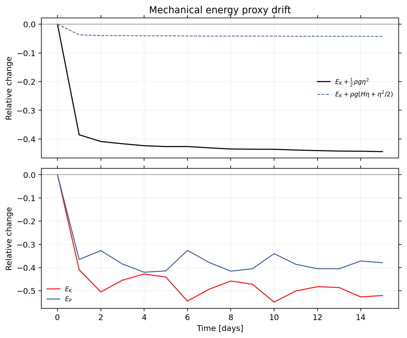
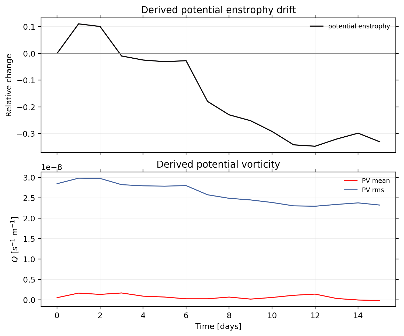
Mass is preserved to roundoff (max |rel| 1.786e-16). The mechanical-energy proxy is not preserved (max |rel| 0.444233). Derived potential enstrophy is not preserved (max |rel| 0.347357).

  • alpha=0: mass preserved to roundoff; quantity not preserved; energy not preserved; PV/enstrophy not preserved
TC6 - Rossby-Haurwitz wave Verified

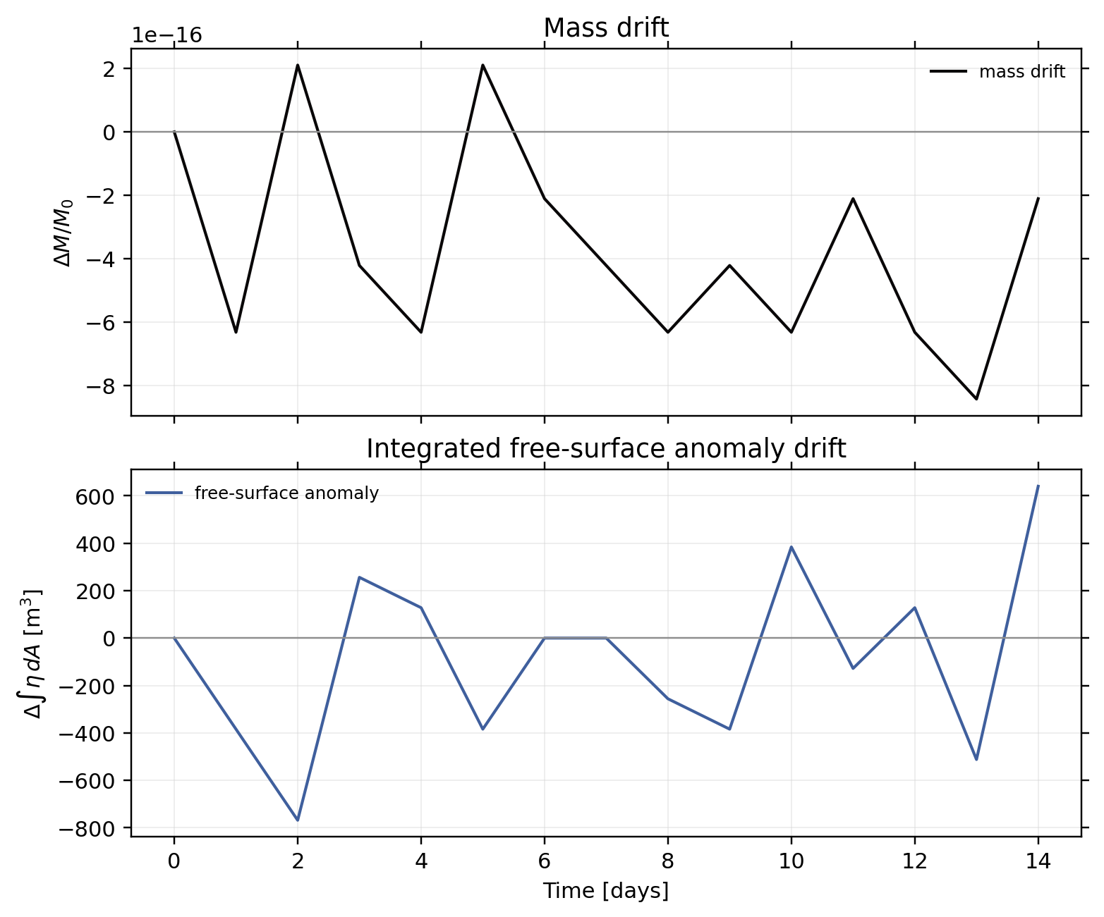
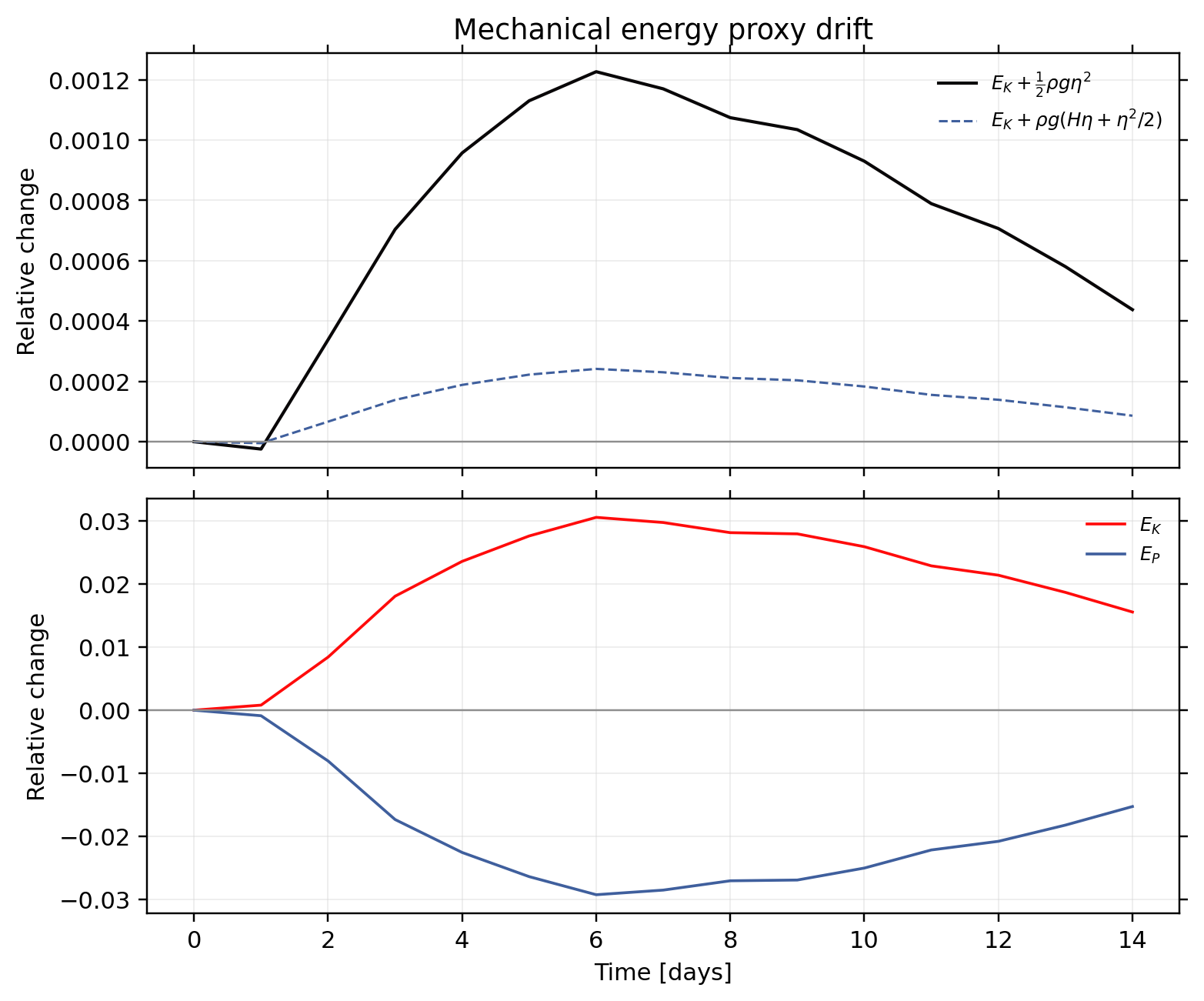
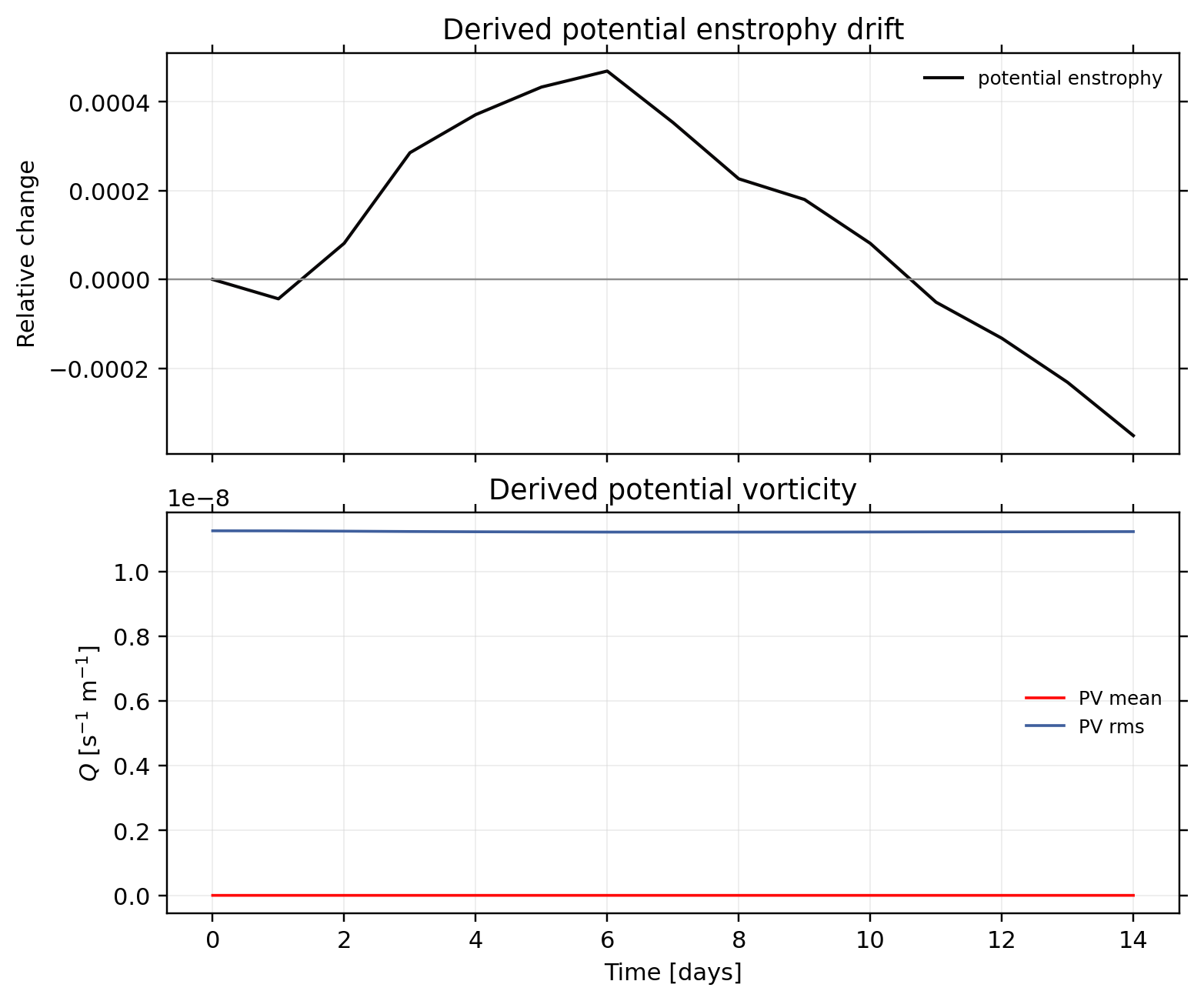
Mass is preserved to roundoff (max |rel| 8.433e-16). The mechanical-energy proxy is not preserved (max |rel| 0.00122662). Derived potential enstrophy is noticeable drift (max |rel| 4.695e-04).

  • alpha=0: mass preserved to roundoff; quantity noticeable drift; energy not preserved; PV/enstrophy noticeable drift
TC7 - Analyzed 500 mb initial state Verified

Mass is preserved to roundoff (max |rel| 1.782e-16). The mechanical-energy proxy is not preserved (max |rel| 0.0114949). Derived potential enstrophy is unavailable (max |rel| n/a).

  • alpha=c1_19781221_0000: mass preserved to roundoff; quantity not a scalar test; energy not preserved; PV/enstrophy unavailable
  • alpha=c2_19790116_0000: mass preserved to roundoff; quantity not a scalar test; energy not preserved; PV/enstrophy unavailable
  • alpha=c3_19790109_0000: mass preserved to roundoff; quantity not a scalar test; energy not preserved; PV/enstrophy unavailable

Williamson TC1: Advection of Cosine Bell Verified

Alphas4
Fields5
Key Days0, 3, 6, 9, 10, 12
Diagnosis Assets84

Definition

Passive advection of a compact cosine bell by solid-body rotation on the sphere. The rotation axis can be tilted relative to the latitude-longitude grid, so the bell can cross the coordinate poles.

What This Test Measures

This is the clean transport test: conservation, phase accuracy, numerical diffusion, overshoots/undershoots, and the ability to move a compact structure through polar coordinate singularities without distortion.

Expected Output

After one 12-day revolution the bell should return to its starting location. The exact and MITgcm contours should nearly overlap, the tracer integral should stay flat, and signed-error contours should remain small and symmetric rather than growing long noisy tails.

Initial Conditions

The tracer is a bell centered at (λc,θc)=(3π/2,0) with compact radius R=a/3:

\[q=\frac{q_0}{2}\left[1+\cos\left(\frac{\pi r}{R}\right)\right],\quad r
\[q=0,\quad r\ge R\]
\[\frac{Dq}{Dt}=\frac{\partial q}{\partial t}+\mathbf{v}\cdot\nabla_s q=0\]

The prescribed velocity is the TC2 solid-body field, but momentum is not stepped in this local MITgcm case.

Python initial-condition script
#%%
from pathlib import Path
import numpy as np

# Grid / constants
NX = 1440
NY = 720
DLON_DEG = 360.0 / NX
DLAT_DEG = 180.0 / NY

R_EARTH = 6.371e6
DAY = 86400.0

# MITgcm ocean bathymetry is negative below sea level.
BATHYMETRY = -4000.0
BATHYMETRY_FILENAME = "bathymetry_flat4000.bin"

# TC1 parameters
U0 = 2.0 * np.pi * R_EARTH / (12.0 * DAY)
H0 = 1000.0               # passive-tracer amplitude
RADIUS_RAD = 1.0 / 3.0    # angular radius
LAT0_DEG = 0.0
LON0_DEG = 270.0          # 3*pi/2
ALPHA_RAD = 1.5707963267948966
#4 cases: [0.0 , 0.05 ,1.5207963267948966 , 1.5707963267948966]

def write_flat_bathymetry(base_dir: Path):
    bathymetry = np.full((NY, NX), BATHYMETRY, dtype=">f4")
    bathymetry.tofile(base_dir / BATHYMETRY_FILENAME)
    print(
        f"Wrote {BATHYMETRY_FILENAME}: bathymetry={BATHYMETRY} m"
    )

def grid_centers():
    lon = (np.arange(NX, dtype=np.float64) + 0.5) * DLON_DEG
    lat = -90.0 + (np.arange(NY, dtype=np.float64) + 0.5) * DLAT_DEG
    return np.meshgrid(lon, lat, indexing="xy")

def spherical_distance_rad(lon_deg, lat_deg, lon0_deg, lat0_deg):
    lon = np.deg2rad(lon_deg)
    lat = np.deg2rad(lat_deg)
    lon0 = np.deg2rad(lon0_deg)
    lat0 = np.deg2rad(lat0_deg)

    dlon = (lon - lon0 + np.pi) % (2.0 * np.pi) - np.pi

    cos_r = (
        np.sin(lat) * np.sin(lat0)
        + np.cos(lat) * np.cos(lat0) * np.cos(dlon)
    )

    return np.arccos(np.clip(cos_r, -1.0, 1.0))

def write_field(base_dir: Path, name: str, field: np.ndarray):
    field.astype(">f4").tofile(base_dir / name)
    print(f"Wrote {name}: min={field.min():.6e}, max={field.max():.6e}")

def streamfunction(lon_rad, lat_rad, alpha_rad):
    return U0 * R_EARTH * (
        np.cos(alpha_rad) * np.sin(lat_rad)
        - np.sin(alpha_rad) * np.cos(lat_rad) * np.cos(lon_rad)
    )

def make_tc1_fields(alpha_rad: float = 0.0):
    lon2d, lat2d = grid_centers()

    # Cosine bell at tracer-cell centers.
    r = spherical_distance_rad(lon2d, lat2d, LON0_DEG, LAT0_DEG)

    tracer = np.zeros((NY, NX), dtype=np.float64)
    inside = r < RADIUS_RAD
    tracer[inside] = 0.5 * H0 * (
        1.0 + np.cos(np.pi * r[inside] / RADIUS_RAD)
    )

    # Derive C-grid face velocities from a streamfunction so their
    # finite-volume divergence vanishes to roundoff.
    lon_u = np.deg2rad(np.arange(NX, dtype=np.float64) * DLON_DEG)
    lat_s = np.deg2rad(-90.0 + np.arange(NY, dtype=np.float64) * DLAT_DEG)
    lat_n = lat_s + np.deg2rad(DLAT_DEG)
    dy = R_EARTH * np.deg2rad(DLAT_DEG)

    psi_n = streamfunction(lon_u[None, :], lat_n[:, None], alpha_rad)
    psi_s = streamfunction(lon_u[None, :], lat_s[:, None], alpha_rad)
    u = (psi_n - psi_s) / dy

    lon_w = np.deg2rad(np.arange(NX, dtype=np.float64) * DLON_DEG)
    lon_e = np.roll(lon_w, -1)
    lat_v = np.deg2rad(-90.0 + np.arange(NY, dtype=np.float64) * DLAT_DEG)
    dx = R_EARTH * np.cos(lat_v) * np.deg2rad(DLON_DEG)

    psi_w = streamfunction(lon_w[None, :], lat_v[:, None], alpha_rad)
    psi_e = streamfunction(lon_e[None, :], lat_v[:, None], alpha_rad)
    v = np.zeros((NY, NX), dtype=np.float64)
    non_polar = np.abs(dx) > 1.0e-14
    v[non_polar, :] = (
        psi_w[non_polar, :] - psi_e[non_polar, :]
    ) / dx[non_polar, None]

    return tracer, u, v

def main():
    base_dir = Path(__file__).resolve().parent

    write_flat_bathymetry(base_dir)

    tracer, u, v = make_tc1_fields(alpha_rad=ALPHA_RAD)

    write_field(base_dir, "S_init.bin", tracer)
    write_field(base_dir, "u_init.bin", u)
    write_field(base_dir, "v_init.bin", v)

    print("Done.")

if __name__ == "__main__":
    main()

# %%

Parameters

  • a=6.371e6 m, g=9.81 m s^-2, Ω=7.292e-5 s^-1 in the local runs.
  • q0=1000, R=a/3, U0=2πa/(12 days).
  • Rendered tilt angles: α=0, 0.05, 1.52, 1.57 rad.
Numerical settings
α=0

Time Step And CFL

alphanTimeStepsdeltaT [s]total [s]max initial CFLstatussource
0172806010368000.0833OKrun-local data

Numerical Settings

rhoConst[kg m-3]gravity[m s-2]deltaT[s]nTimeSteps[steps]delR[m]delX[deg]delY[deg]
1000.9.8160.0172804000.1440*0.25720*0.25

Grid And MPI Layout

sNx[cells]sNy[cells]nPx[MPI tiles]nPy[MPI tiles]Nx[cells]Ny[cells]mpi_ranks[ranks]
120180124144072048
α=0.05

Time Step And CFL

alphanTimeStepsdeltaT [s]total [s]max initial CFLstatussource
0.051036801010368000.332OKrun-local data

Numerical Settings

rhoConst[kg m-3]gravity[m s-2]deltaT[s]nTimeSteps[steps]delR[m]delX[deg]delY[deg]
1000.9.8110.01036804000.1440*0.25720*0.25

Grid And MPI Layout

sNx[cells]sNy[cells]nPx[MPI tiles]nPy[MPI tiles]Nx[cells]Ny[cells]mpi_ranks[ranks]
120180124144072048
α=1.52

Time Step And CFL

alphanTimeStepsdeltaT [s]total [s]max initial CFLstatussource
1.5213824000.7510368000.49OKrun-local data

Numerical Settings

rhoConst[kg m-3]gravity[m s-2]deltaT[s]nTimeSteps[steps]delR[m]delX[deg]delY[deg]
1000.9.810.7513824004000.1440*0.25720*0.25

Grid And MPI Layout

sNx[cells]sNy[cells]nPx[MPI tiles]nPy[MPI tiles]Nx[cells]Ny[cells]mpi_ranks[ranks]
120180124144072048
α=1.57

Time Step And CFL

alphanTimeStepsdeltaT [s]total [s]max initial CFLstatussource
1.5713824000.7510368000.478OKrun-local data

Numerical Settings

rhoConst[kg m-3]gravity[m s-2]deltaT[s]nTimeSteps[steps]delR[m]delX[deg]delY[deg]
1000.9.810.7513824004000.1440*0.25720*0.25

Grid And MPI Layout

sNx[cells]sNy[cells]nPx[MPI tiles]nPy[MPI tiles]Nx[cells]Ny[cells]mpi_ranks[ranks]
120180124144072048

TC1 passive tracer: key-day snapshots

Rendered days: 0, 3, 6, 9, 10, 12.

Units: Passive Tracer [psu], ETAN [m], PsiVEL [m3 s-1], PhiVEL [m2 s-1], Velocity Magnitude [m s-1].

α=0
alpha 0, ETAN, Day 0
alpha 0, ETAN, Day 3
alpha 0, ETAN, Day 6
alpha 0, ETAN, Day 9
alpha 0, ETAN, Day 10
α=0.05
alpha 0.05, ETAN, Day 0
alpha 0.05, ETAN, Day 3
alpha 0.05, ETAN, Day 6
alpha 0.05, ETAN, Day 9
alpha 0.05, ETAN, Day 10
α=1.52
alpha 1.52, ETAN, Day 0
alpha 1.52, ETAN, Day 3
alpha 1.52, ETAN, Day 6
alpha 1.52, ETAN, Day 9
alpha 1.52, ETAN, Day 10
α=1.57
alpha 1.57, ETAN, Day 0
alpha 1.57, ETAN, Day 3
alpha 1.57, ETAN, Day 6
alpha 1.57, ETAN, Day 9
alpha 1.57, ETAN, Day 10

Existing tutorials in MITgcm: advect_cs

Definition

verification/advect_cs is a cubed-sphere passive-tracer advection tutorial. Here it is staged as a Williamson TC1 analogue: prescribed 12-day solid-body velocity, four rotation angles, and no momentum stepping.

What This Test Measures

It isolates cubed-sphere passive-tracer transport: phase error, numerical diffusion, face-edge continuity, and tracer conservation under prescribed velocity.

Expected Output

The tracer should return close to its initial bell after one revolution. Eta is not the target field; this existing tutorial tests transport, not free-surface dynamics.

Initial Conditions

S.init is the active passive tracer: a compact cosine bell centered at lon 180 deg, lat 35 deg, radius 0.3 chord units. T.init is an additional tracer from the original tutorial.

MITgcm tutorial input generator
for tl=1:6,
%lon(:,tl,:)=rdda(sprintf('LONC.%3.3i.bin',tl),[32 32],1,'real*8','b')*pi/180;
%lat(:,tl,:)=rdda(sprintf('LATC.%3.3i.bin',tl),[32 32],1,'real*8','b')*pi/180;
 xx=rdda(sprintf('grid_cs32.face%3.3i.bin',tl),[33 33],1,'real*8','b');
 lon(:,tl,:)=xx(1:32,1:32)*pi/180;
 xx=rdda(sprintf('grid_cs32.face%3.3i.bin',tl),[33 33],2,'real*8','b');
 lat(:,tl,:)=xx(1:32,1:32)*pi/180;
end
X=cos(lat).*sin(lon);Y=-cos(lat).*cos(lon);Z=sin(lat);clear lat lon

%lon0=-90  *pi/180;
lon0=+90  *pi/180;
lat0=  0  *pi/180;
xo=cos(lat0).*sin(lon0);yo=-cos(lat0).*cos(lon0);zo=sin(lat0);
ro=0.3;
R=sqrt( (X-xo).^2 + (Y-yo).^2 + (Z-zo).^2 );
t=1+(1+cos( pi*min(R/ro,1+0*R) ))/2;
fid=fopen('T.init','w','b');
fwrite(fid,t(:),'real*8');
fclose(fid)

%lon0=  0  *pi/180;
lon0=180  *pi/180;
lat0=35   *pi/180;
xo=cos(lat0).*sin(lon0);yo=-cos(lat0).*cos(lon0);zo=sin(lat0);
ro=0.3;
R=sqrt( (X-xo).^2 + (Y-yo).^2 + (Z-zo).^2 );
s=1+(1+cos( pi*min(R/ro,1+0*R) ))/2;
fid=fopen('S.init','w','b');
fwrite(fid,s(:),'real*8');
fclose(fid)

lon0=0    *pi/180;
lat0=0    *pi/180;
xo=cos(lat0).*sin(lon0);yo=-cos(lat0).*cos(lon0);zo=sin(lat0);
ro=0.3;
R=sqrt( (X-xo).^2 + (Y-yo).^2 + (Z-zo).^2 );
h=1e4*(1+cos( pi*min(R/ro,1+0*R) ))/2; %cosine bell
%h=1e4*(1-( min(R/ro,1+0*R) ))/2;	%cone
%fid=fopen('mountain_eq.init','w','b');
%fwrite(fid,h(:),'real*8');
%fclose(fid)

lon0=0    *pi/180;
lat0=30   *pi/180;
xo=cos(lat0).*sin(lon0);yo=-cos(lat0).*cos(lon0);zo=sin(lat0);
ro=0.3;
R=sqrt( (X-xo).^2 + (Y-yo).^2 + (Z-zo).^2 );
h=1e4*(1+cos( pi*min(R/ro,1+0*R) ))/2; %cosine bell
%h=1e4*(1-( min(R/ro,1+0*R) ))/2;	%cone
%fid=fopen('mountain_30.init','w','b');
%fwrite(fid,h(:),'real*8');
%fclose(fid)

Parameters

  • Grid: CS32 cubed sphere, six faces, six MPI ranks.
  • Velocity: 12-day solid-body rotation from ini_vel.F, with alpha read from tc1_alpha.txt.
  • Angles: 0, 0.05, 1.52, 1.57 rad.
Numerical settings by alpha
α=0

Time Step And CFL

alphanTimeStepsdeltaT [s]total [s]max initial CFLstatussource
0—27001036800——run-local data

Numerical Settings

rhoConst[kg m-3]gravity[m s-2]deltaT[s]nTimeSteps[steps]delR[m]delX[deg]delY[deg]
——2700.—1.E5——

Grid And MPI Layout

sNx[cells]sNy[cells]nPx[MPI tiles]nPy[MPI tiles]Nx[cells]Ny[cells]mpi_ranks[ranks]
32322364966
α=0.05

Time Step And CFL

alphanTimeStepsdeltaT [s]total [s]max initial CFLstatussource
0.05—27001036800——run-local data

Numerical Settings

rhoConst[kg m-3]gravity[m s-2]deltaT[s]nTimeSteps[steps]delR[m]delX[deg]delY[deg]
——2700.—1.E5——

Grid And MPI Layout

sNx[cells]sNy[cells]nPx[MPI tiles]nPy[MPI tiles]Nx[cells]Ny[cells]mpi_ranks[ranks]
32322364966
α=1.52

Time Step And CFL

alphanTimeStepsdeltaT [s]total [s]max initial CFLstatussource
1.52—27001036800——run-local data

Numerical Settings

rhoConst[kg m-3]gravity[m s-2]deltaT[s]nTimeSteps[steps]delR[m]delX[deg]delY[deg]
——2700.—1.E5——

Grid And MPI Layout

sNx[cells]sNy[cells]nPx[MPI tiles]nPy[MPI tiles]Nx[cells]Ny[cells]mpi_ranks[ranks]
32322364966
α=1.57

Time Step And CFL

alphanTimeStepsdeltaT [s]total [s]max initial CFLstatussource
1.57—27001036800——run-local data

Numerical Settings

rhoConst[kg m-3]gravity[m s-2]deltaT[s]nTimeSteps[steps]delR[m]delX[deg]delY[deg]
——2700.—1.E5——

Grid And MPI Layout

sNx[cells]sNy[cells]nPx[MPI tiles]nPy[MPI tiles]Nx[cells]Ny[cells]mpi_ranks[ranks]
32322364966

Rendered days: 0, 3, 6, 9, 10, 12. Shown PNGs are lat-lon interpolations when available; native cube-net plots are retained separately.

α=0
Error
advect_cs alpha 0, Passive Tracer, Day 0
advect_cs alpha 0, Passive Tracer, Day 3
advect_cs alpha 0, Passive Tracer, Day 6
advect_cs alpha 0, Passive Tracer, Day 9
advect_cs alpha 0, Passive Tracer, Day 10
advect_cs alpha 0, Passive Tracer, Day 12
α=0.05
Error
advect_cs alpha 0.05, Passive Tracer, Day 0
advect_cs alpha 0.05, Passive Tracer, Day 3
advect_cs alpha 0.05, Passive Tracer, Day 6
advect_cs alpha 0.05, Passive Tracer, Day 9
advect_cs alpha 0.05, Passive Tracer, Day 10
advect_cs alpha 0.05, Passive Tracer, Day 12
α=1.52
Error
advect_cs alpha 1.52, Passive Tracer, Day 0
advect_cs alpha 1.52, Passive Tracer, Day 3
advect_cs alpha 1.52, Passive Tracer, Day 6
advect_cs alpha 1.52, Passive Tracer, Day 9
advect_cs alpha 1.52, Passive Tracer, Day 10
advect_cs alpha 1.52, Passive Tracer, Day 12
α=1.57
Error
advect_cs alpha 1.57, Passive Tracer, Day 0
advect_cs alpha 1.57, Passive Tracer, Day 3
advect_cs alpha 1.57, Passive Tracer, Day 6
advect_cs alpha 1.57, Passive Tracer, Day 9
advect_cs alpha 1.57, Passive Tracer, Day 10
advect_cs alpha 1.57, Passive Tracer, Day 12
Results: existing MITgcm tutorial advect_cs - Error analysis and diagnosis assets

Errors are model passive tracer minus the advected analytic bell.

α=0
advect_cs alpha 0, error norms
advect_cs alpha 0, final model tracer
advect_cs alpha 0, final exact tracer
advect_cs alpha 0, final tracer error
advect_cs alpha 0, postprocessing tracer integral
advect_cs alpha 0, postprocessing velocity
Ready data files
α=0.05
advect_cs alpha 0.05, error norms
advect_cs alpha 0.05, final model tracer
advect_cs alpha 0.05, final exact tracer
advect_cs alpha 0.05, final tracer error
advect_cs alpha 0.05, postprocessing tracer integral
advect_cs alpha 0.05, postprocessing velocity
Ready data files
α=1.52
advect_cs alpha 1.52, error norms
advect_cs alpha 1.52, final model tracer
advect_cs alpha 1.52, final exact tracer
advect_cs alpha 1.52, final tracer error
advect_cs alpha 1.52, postprocessing tracer integral
advect_cs alpha 1.52, postprocessing velocity
Ready data files
α=1.57
advect_cs alpha 1.57, error norms
advect_cs alpha 1.57, final model tracer
advect_cs alpha 1.57, final exact tracer
advect_cs alpha 1.57, final tracer error
advect_cs alpha 1.57, postprocessing tracer integral
advect_cs alpha 1.57, postprocessing velocity
Ready data files
General
Ready data files

Williamson TC2: Global Steady-State Nonlinear Zonal Geostrophic Flow Verified

Alphas4
Fields5
Key Days0, 3, 6, 9, 10, 12
Diagnosis Assets36

Definition

A full nonlinear shallow-water steady state: global solid-body zonal flow balanced by the free-surface height field. The flow is exact for every time when the continuous balance is preserved.

What This Test Measures

Balanced nonlinear dynamics, metric terms, Coriolis terms, pole treatment, and preservation of a known steady state. The paper also identifies TC2 as the performance benchmark, typically using α=π/4 for a 5-day run.

Expected Output

A good run stays almost motionless in the rotating balance: height and velocity errors should remain near discretization error, with little gravity-wave noise. Mesh refinement should reduce the 5-day error norms cleanly.

Initial Conditions And Equations

The active Williamson cases are run as one-layer rotating shallow-water problems. The MITgcm fields reduce to horizontal velocity u=(u,v) and free surface η over depth H.

\[\frac{D\mathbf{u}}{Dt}+f\hat{k}\times\mathbf{u}=-g\nabla_s\eta+\mathcal{D}_{\mathbf{u}}+\mathbf{F}\]
\[\frac{\partial \eta}{\partial t}+\nabla_s\cdot[(H+\eta)\mathbf{u}]=S_{\eta}\]
\[\frac{Dq}{Dt}=\mathcal{D}_{q}+S_q \quad \text{when passive tracers are enabled}\]

Each testcase changes the analytic initial state, forcing, bathymetry, or expected diagnostic behavior of this same system.

With longitude λ, latitude θ, and tilt α:

\[u=U_0\left(\cos\theta\cos\alpha+\cos\lambda\sin\theta\sin\alpha\right)\]
\[v=-U_0\sin\lambda\sin\alpha\]
\[\mu=-\cos\lambda\cos\theta\sin\alpha+\sin\theta\cos\alpha\]
\[g h=g h_0-\left(a\Omega U_0+\frac{1}{2}U_0^2\right)\mu^2\]
Python initial-condition script
#%%
from pathlib import Path
import sys
import numpy as np

SCRIPTS_DIR = Path(__file__).resolve().parent.parent.parent / "Scripts"
if str(SCRIPTS_DIR) not in sys.path:
    sys.path.insert(0, str(SCRIPTS_DIR))

import williamson_cube as wc

# ============================================================
# Williamson TC2: Global steady-state nonlinear zonal geostrophic flow
# Clean MITgcm initializer for one-layer spherical shallow water
# ============================================================

# Grid
NX = 1440
NY = 720
DLON_RAD = 2.0 * np.pi / NX
DLAT_RAD = np.pi / NY

# Physical constants
R_EARTH = 6.371e6
OMEGA = 7.292e-5
G = 9.81

# Standard Williamson TC2 constants
DAY = 86400.0
U0 = 2.0 * np.pi * R_EARTH / (12.0 * DAY)   # one revolution in 12 days
GH0 = 2.94e4                                # m^2/s^2
H0 = GH0 / G                                # mean layer depth in meters

# Rotation angle. The job scripts patch ALPHA_RAD in the run-local copy
# before this generator writes the initial fields.
ALPHA_RAD = 0.0

# Output files
BATHY_FILE = "bathymetry_flat4000.bin"
ETA_FILE = "eta_init.bin"
U_FILE = "u_init.bin"
V_FILE = "v_init.bin"
FCORI_C_FILE = "fCoriC.bin"
FCORI_G_FILE = "fCoriG.bin"
FCORI_COS_FILE = "fCorCs.bin"

def write_field(base_dir: Path, name: str, field: np.ndarray) -> None:
    field.astype(">f4").tofile(base_dir / name)
    print(f"Wrote {name}: shape={field.shape}, min={field.min():.6e}, max={field.max():.6e}")

def grid_cell_centers():
    """
    C-cell centers:
      lon_c = (i+1/2) dlon
      lat_c = -pi/2 + (j+1/2) dlat
    """
    lon_c = (np.arange(NX, dtype=np.float64) + 0.5) * DLON_RAD
    lat_c = -0.5 * np.pi + (np.arange(NY, dtype=np.float64) + 0.5) * DLAT_RAD
    return np.meshgrid(lon_c, lat_c, indexing="xy")

def grid_u_faces():
    """
    U faces:
      lon_u = i dlon
      lat_u = cell-center latitude
    """
    lon_u = np.arange(NX, dtype=np.float64) * DLON_RAD
    lat_u = -0.5 * np.pi + (np.arange(NY, dtype=np.float64) + 0.5) * DLAT_RAD
    return np.meshgrid(lon_u, lat_u, indexing="xy")

def grid_v_faces():
    """
    V faces:
      lon_v = cell-center longitude
      lat_v = -pi/2 + j dlat
    """
    lon_v = (np.arange(NX, dtype=np.float64) + 0.5) * DLON_RAD
    lat_v = -0.5 * np.pi + np.arange(NY, dtype=np.float64) * DLAT_RAD
    return np.meshgrid(lon_v, lat_v, indexing="xy")

def grid_corners():
    """
    Grid corners used by MITgcm's fCoriG read path.
    """
    lon_g = np.arange(NX, dtype=np.float64) * DLON_RAD
    lat_g = -0.5 * np.pi + np.arange(NY, dtype=np.float64) * DLAT_RAD
    return np.meshgrid(lon_g, lat_g, indexing="xy")

def rotated_mu(lon_rad: np.ndarray, lat_rad: np.ndarray, alpha_rad: float) -> np.ndarray:
    return (
        -np.cos(lon_rad) * np.cos(lat_rad) * np.sin(alpha_rad)
        + np.sin(lat_rad) * np.cos(alpha_rad)
    )

def write_flat_bathymetry(base_dir: Path) -> None:
    bathy = np.full((NY, NX), -H0, dtype=">f4")
    bathy.tofile(base_dir / BATHY_FILE)
    print(f"Wrote {BATHY_FILE} with constant depth {-H0:.6f} m")

def write_rotated_coriolis(base_dir: Path, alpha_rad: float = ALPHA_RAD) -> None:
    lon_c, lat_c = grid_cell_centers()
    lon_g, lat_g = grid_corners()

    mu_c = rotated_mu(lon_c, lat_c, alpha_rad)
    mu_g = rotated_mu(lon_g, lat_g, alpha_rad)

    write_field(base_dir, FCORI_C_FILE, 2.0 * OMEGA * mu_c)
    write_field(base_dir, FCORI_G_FILE, 2.0 * OMEGA * mu_g)
    write_field(
        base_dir,
        FCORI_COS_FILE,
        2.0 * OMEGA * np.sqrt(np.maximum(0.0, 1.0 - mu_c * mu_c)),
    )

def make_tc2_eta(alpha_rad: float = ALPHA_RAD):
    """
    Cell-center free-surface anomaly eta = h - H0,
    with h from the Williamson TC2 analytic height field.
    """
    lon_c, lat_c = grid_cell_centers()

    mu = (
        -np.cos(lon_c) * np.cos(lat_c) * np.sin(alpha_rad)
        + np.sin(lat_c) * np.cos(alpha_rad)
    )

    gh = GH0 - (R_EARTH * OMEGA * U0 + 0.5 * U0**2) * mu**2
    h = gh / G
    eta = h - H0

    return eta

def make_tc2_u(alpha_rad: float = ALPHA_RAD):
    """
    Zonal-face velocity from the paper formula.
    """
    lon_u, lat_u = grid_u_faces()

    u = U0 * (
        np.cos(lat_u) * np.cos(alpha_rad)
        + np.cos(lon_u) * np.sin(lat_u) * np.sin(alpha_rad)
    )

    return u

def make_tc2_v(alpha_rad: float = ALPHA_RAD):
    """
    Meridional-face velocity from the paper formula.
    """
    lon_v, lat_v = grid_v_faces()

    v = -U0 * np.sin(lon_v) * np.sin(alpha_rad)

    # Pole rows are coordinate-singular V-faces on the lat-lon grid.
    # Set them to zero for a clean MITgcm initialization.
    v[0, :] = 0.0
    v[-1, :] = 0.0

    return v

def main():
    base_dir = Path(__file__).resolve().parent
    if not (base_dir / ".use_latlon_grid").exists():
        wc.generate_tc2(base_dir, alpha_rad=ALPHA_RAD)
        print("")
        print("Done.")
        print(f"ALPHA_RAD = {ALPHA_RAD:.16g}")
        print(f"ALPHA_DEG = {np.rad2deg(ALPHA_RAD):.16g}")
        print(f"U0        = {U0:.12f} m/s")
        print(f"H0        = {H0:.12f} m")
        print(f"GH0       = {GH0:.12f} m^2/s^2")
        return

    write_flat_bathymetry(base_dir)
    write_rotated_coriolis(base_dir, alpha_rad=ALPHA_RAD)
    eta = make_tc2_eta(alpha_rad=ALPHA_RAD)
    u = make_tc2_u(alpha_rad=ALPHA_RAD)
    v = make_tc2_v(alpha_rad=ALPHA_RAD)

    write_field(base_dir, ETA_FILE, eta)
    write_field(base_dir, U_FILE, u)
    write_field(base_dir, V_FILE, v)

    print("")
    print("Done.")
    print(f"ALPHA_RAD = {ALPHA_RAD:.16g}")
    print(f"ALPHA_DEG = {np.rad2deg(ALPHA_RAD):.16g}")
    print(f"U0        = {U0:.12f} m/s")
    print(f"H0        = {H0:.12f} m")
    print(f"GH0       = {GH0:.12f} m^2/s^2")

if __name__ == "__main__":
    main()

# %%

Parameters

  • U0=2πa/(12 days).
  • g h0=2.94e4 m^2 s^-2, so local H0=g h0/g=2996.94 m.
  • Standard tilts: α=0, 0.05, π/2-0.05, π/2; local outputs use 0, 0.05, 1.52, 1.57 rad.

Validation Result

Validation is complete for the four local tilt cases. Alpha 0 uses the unrotated lat-lon run; alpha 0.05, 1.52, and 1.57 use the regenerated rotated-Coriolis 12-day runs with selectCoriMap=3 and the rotated fCoriC/fCoriG/fCorCs files. All saved postprocessing fields remain finite, with mass preserved to roundoff. Day-12 error norms are steady for the corrected outputs: L2_eta=2.42e-7, L2_u=4.03e-7, L2_v=6.29e-6 at alpha 0; L2_eta=4.17e-5, L2_u=2.34e-4, L2_v=4.75e-3 at alpha 0.05; L2_eta=2.98e-4, L2_u=8.74e-3, L2_v=1.33e-1 at alpha 1.52; and L2_eta=2.93e-4, L2_u=1.35e-2, L2_v=2.11e-1 at alpha 1.57.

Numerical settings
α=0

Time Step And CFL

alphanTimeStepsdeltaT [s]total [s]max initial CFLstatussource
0172806010368000.0833OKrun-local data

Numerical Settings

rhoConst[kg m-3]gravity[m s-2]deltaT[s]nTimeSteps[steps]delR[m]delX[deg]delY[deg]
1.9.8160.0172802996.94189602446461440*0.25720*0.25

Grid And MPI Layout

sNx[cells]sNy[cells]nPx[MPI tiles]nPy[MPI tiles]Nx[cells]Ny[cells]mpi_ranks[ranks]
18012086144072048
α=0.05

Time Step And CFL

alphanTimeStepsdeltaT [s]total [s]max initial CFLstatussource
0.051036801010368000.332OKrun-local data

Numerical Settings

rhoConst[kg m-3]gravity[m s-2]deltaT[s]nTimeSteps[steps]delR[m]delX[deg]delY[deg]
1.9.8110.01036802996.94189602446461440*0.25720*0.25

Grid And MPI Layout

sNx[cells]sNy[cells]nPx[MPI tiles]nPy[MPI tiles]Nx[cells]Ny[cells]mpi_ranks[ranks]
18012086144072048
α=1.52

Time Step And CFL

alphanTimeStepsdeltaT [s]total [s]max initial CFLstatussource
1.521036800110368000.636checkrun-local data

Numerical Settings

rhoConst[kg m-3]gravity[m s-2]deltaT[s]nTimeSteps[steps]delR[m]delX[deg]delY[deg]
1.9.811.010368002996.94189602446461440*0.25720*0.25

Grid And MPI Layout

sNx[cells]sNy[cells]nPx[MPI tiles]nPy[MPI tiles]Nx[cells]Ny[cells]mpi_ranks[ranks]
18012086144072048
α=1.57

Time Step And CFL

alphanTimeStepsdeltaT [s]total [s]max initial CFLstatussource
1.5720736000.510368000.318OKrun-local data

Numerical Settings

rhoConst[kg m-3]gravity[m s-2]deltaT[s]nTimeSteps[steps]delR[m]delX[deg]delY[deg]
1.9.810.520736002996.94189602446461440*0.25720*0.25

Grid And MPI Layout

sNx[cells]sNy[cells]nPx[MPI tiles]nPy[MPI tiles]Nx[cells]Ny[cells]mpi_ranks[ranks]
18012086144072048

vortexSphere_Williamson_TC2: key-day snapshots

Rendered days: 0, 3, 6, 9, 10, 12.

Units: Eta [m], ETAN [m], PsiVEL [m3 s-1], PhiVEL [m2 s-1], Velocity Magnitude [m s-1].

α=0
alpha 0, Eta, Day 0
alpha 0, Eta, Day 3
alpha 0, Eta, Day 6
alpha 0, Eta, Day 9
alpha 0, Eta, Day 10
alpha 0, Eta, Day 12
α=0.05
alpha 0.05, Eta, Day 0
alpha 0.05, Eta, Day 3
alpha 0.05, Eta, Day 6
alpha 0.05, Eta, Day 9
alpha 0.05, Eta, Day 10
alpha 0.05, Eta, Day 12
α=1.52
alpha 1.52, Eta, Day 0
alpha 1.52, Eta, Day 3
alpha 1.52, Eta, Day 6
alpha 1.52, Eta, Day 9
alpha 1.52, Eta, Day 10
alpha 1.52, Eta, Day 12
α=1.57
alpha 1.57, Eta, Day 0
alpha 1.57, Eta, Day 3
alpha 1.57, Eta, Day 6
alpha 1.57, Eta, Day 9
alpha 1.57, Eta, Day 10
alpha 1.57, Eta, Day 12

Williamson TC3: Steady Geostrophic Flow with Compact Support Validated with caveat

Alphas2
Fields5
Key Days0, 1, 2, 3, 4, 5
Diagnosis Assets18

Definition

A steady nonlinear geostrophic flow like TC2, but the wind is a smooth compact jet. The active balanced flow occupies only a limited latitudinal band.

What This Test Measures

Whether a model can maintain a localized balanced flow without leakage, phase drift, ringing near smooth compact-support edges, or spurious gravity waves.

Expected Output

The compact jet and free-surface anomaly should stay steady. Errors should be localized near the jet edges if they appear at all, and conservation diagnostics should show little long-term drift.

Initial Conditions And Equations

The active Williamson cases are run as one-layer rotating shallow-water problems. The MITgcm fields reduce to horizontal velocity u=(u,v) and free surface η over depth H.

\[\frac{D\mathbf{u}}{Dt}+f\hat{k}\times\mathbf{u}=-g\nabla_s\eta+\mathcal{D}_{\mathbf{u}}+\mathbf{F}\]
\[\frac{\partial \eta}{\partial t}+\nabla_s\cdot[(H+\eta)\mathbf{u}]=S_{\eta}\]
\[\frac{Dq}{Dt}=\mathcal{D}_{q}+S_q \quad \text{when passive tracers are enabled}\]

Each testcase changes the analytic initial state, forcing, bathymetry, or expected diagnostic behavior of this same system.

The local implementation builds the velocity from a compact bump in rotated latitude θ' and computes the height by integrating the nonlinear geostrophic balance:

\[u'=U_0 B(\theta'),\quad v'=0\]
\[B(\theta')=0\quad \text{outside }[-\pi/6,\pi/2]\]
\[h=H_0+\int \text{balanced pressure-gradient contribution}\,d\theta'\]
Python initial-condition script
#!/usr/bin/env python3
from __future__ import annotations

from pathlib import Path
import sys

import numpy as np

SCRIPTS_DIR = Path(__file__).resolve().parent.parent.parent / "Scripts"
if str(SCRIPTS_DIR) not in sys.path:
    sys.path.insert(0, str(SCRIPTS_DIR))

import williamson_fields as wf
import williamson_cube as wc

NX = wf.NX
NY = wf.NY
R_EARTH = wf.R_EARTH
G = wf.G
H0 = wf.H0_SOLID
ALPHA_RAD = 0.0

BATHY_FILE = "bathymetry_flat_tc3.bin"
ETA_FILE = "eta_init.bin"
U_FILE = "u_init.bin"
V_FILE = "v_init.bin"
FCORI_C_FILE = "fCoriC.bin"
FCORI_G_FILE = "fCoriG.bin"
FCORI_COS_FILE = "fCorCs.bin"


def make_bathymetry() -> object:
    return wf.flat_bathymetry(H0)


def grid_corners() -> tuple[object, object]:
    lon = np.arange(NX, dtype=np.float64) * wf.DLON_RAD
    lat = -0.5 * np.pi + np.arange(NY, dtype=np.float64) * wf.DLAT_RAD
    return np.meshgrid(lon, lat, indexing="xy")


def rotated_mu(lon_rad: object, lat_rad: object, alpha_rad: float) -> object:
    return (
        -np.cos(lon_rad) * np.cos(lat_rad) * np.sin(alpha_rad)
        + np.sin(lat_rad) * np.cos(alpha_rad)
    )


def write_rotated_coriolis(base_dir: Path, alpha_rad: float = ALPHA_RAD) -> None:
    lon_c, lat_c = wf.grid_cell_centers()
    lon_g, lat_g = grid_corners()
    mu_c = rotated_mu(lon_c, lat_c, alpha_rad)
    mu_g = rotated_mu(lon_g, lat_g, alpha_rad)

    wf.write_field(base_dir, FCORI_C_FILE, 2.0 * wf.OMEGA * mu_c)
    wf.write_field(base_dir, FCORI_G_FILE, 2.0 * wf.OMEGA * mu_g)
    wf.write_field(
        base_dir,
        FCORI_COS_FILE,
        2.0 * wf.OMEGA * np.sqrt(np.maximum(0.0, 1.0 - mu_c * mu_c)),
    )


def make_eta(alpha_rad: float = ALPHA_RAD) -> object:
    lon, lat = wf.grid_cell_centers()
    return wf.tc3_eta(lon, lat, alpha_rad=alpha_rad)


def make_velocity_fields(alpha_rad: float = ALPHA_RAD) -> tuple[object, object]:
    return wf.tc3_velocity_fields(alpha_rad=alpha_rad)


def main() -> None:
    base_dir = Path(__file__).resolve().parent
    if not (base_dir / ".use_latlon_grid").exists():
        wc.generate_tc3(base_dir, alpha_rad=ALPHA_RAD)
        print("")
        print("Done.")
        print(f"ALPHA_RAD = {ALPHA_RAD:.16g}")
        print(f"ALPHA_DEG = {np.rad2deg(ALPHA_RAD):.16g}")
        print(f"H0        = {H0:.12f} m")
        print(f"U0        = {wf.TC3_U0:.12f} m/s")
        print(f"XE        = {wf.TC3_XE:.12f}")
        return

    bathy = make_bathymetry()
    write_rotated_coriolis(base_dir, alpha_rad=ALPHA_RAD)
    eta = make_eta(alpha_rad=ALPHA_RAD)
    u, v = make_velocity_fields(alpha_rad=ALPHA_RAD)

    wf.write_field(base_dir, BATHY_FILE, bathy)
    wf.write_field(base_dir, ETA_FILE, eta)
    wf.write_field(base_dir, U_FILE, u)
    wf.write_field(base_dir, V_FILE, v)
    print("")
    print("Done.")
    print(f"ALPHA_RAD = {ALPHA_RAD:.16g}")
    print(f"ALPHA_DEG = {np.rad2deg(ALPHA_RAD):.16g}")
    print(f"H0        = {H0:.12f} m")
    print(f"U0        = {wf.TC3_U0:.12f} m/s")
    print(f"XE        = {wf.TC3_XE:.12f}")


if __name__ == "__main__":
    main()

Parameters

  • U0=2πa/(12 days), H0=2996.94 m.
  • Compact support interval: θ0=-π/6 to θ1=π/2.
  • Runs can be rotated by α to move the jet away from grid lines.
  • Published c2 uses α=π/3, deltaT=0.5 s, nTimeSteps=864000, selectCoriMap=3, fCoriC/fCoriG/fCorCs, and the 45-rank large-partition Slurm job job_tc3_c2_latlon_rotcori_5day_45rank.slurm.

Validation Result

Validated with caveat. Both published TC3 setups pass preflight and saved fields stay finite. Alpha 0 is clean through day 5 (L2_eta=1.79e-5, L2_u=1.82e-5, L2_v=1.06e-4 m s^-1). The rotated alpha 1.0472 run is finite and correctly staged, but it shows larger steady-state drift (day-5 L2_eta=9.54e-4, L2_u=1.93e-2, L2_v=1.63e-1 m s^-1) and nontrivial energy/PV drift, so it should not be described as a perfect verification pass.

Numerical settings
α=0

Time Step And CFL

alphanTimeStepsdeltaT [s]total [s]max initial CFLstatussource
07200604320000.0969OKrun-local data

Numerical Settings

rhoConst[kg m-3]gravity[m s-2]deltaT[s]nTimeSteps[steps]delR[m]delX[deg]delY[deg]
1.9.8160.072002996.94189602446461440*0.25720*0.25

Grid And MPI Layout

sNx[cells]sNy[cells]nPx[MPI tiles]nPy[MPI tiles]Nx[cells]Ny[cells]mpi_ranks[ranks]
16014495144072045
α=1.0472

Time Step And CFL

alphanTimeStepsdeltaT [s]total [s]max initial CFLstatussource
1.04728640000.54320000.318OKrun-local data

Numerical Settings

rhoConst[kg m-3]gravity[m s-2]deltaT[s]nTimeSteps[steps]delR[m]delX[deg]delY[deg]
1.9.810.58640002996.94189602446461440*0.25720*0.25

Grid And MPI Layout

sNx[cells]sNy[cells]nPx[MPI tiles]nPy[MPI tiles]Nx[cells]Ny[cells]mpi_ranks[ranks]
16014495144072045

vortexSphere_Williamson_TC3: key-day snapshots

Rendered days: 0, 1, 2, 3, 4, 5.

Units: Eta [m], ETAN [m], PsiVEL [m3 s-1], PhiVEL [m2 s-1], Velocity Magnitude [m s-1].

α=0
alpha 0, Eta, Day 0
alpha 0, Eta, Day 1
alpha 0, Eta, Day 2
alpha 0, Eta, Day 3
alpha 0, Eta, Day 4
alpha 0, Eta, Day 5
α=1.0472
alpha 1.0472, Eta, Day 0
alpha 1.0472, Eta, Day 1
alpha 1.0472, Eta, Day 2
alpha 1.0472, Eta, Day 3
alpha 1.0472, Eta, Day 4
alpha 1.0472, Eta, Day 5

Williamson TC4: Forced Nonlinear Translating Low Verified

The required U0=20 and U0=40 m s^-1 runs are complete through day 5; snapshots, conservation, and postprocessing assets are published.

Alphas2
Fields5
Key Days0, 1, 2, 3, 4, 5
Diagnosis Assets23

Definition

A forced nonlinear shallow-water exact-solution test with a translating low. The prescribed forcing makes the unsteady analytic disturbance the target solution.

What This Test Measures

TC4 targets unsteady nonlinear accuracy with a known forced solution: advection of a strong localized low, source-term balance, and error growth in a moving feature.

Expected Output

The translating low should keep its shape as it moves eastward. Both submitted TC4 runs complete normally and keep finite day-5 state fields. The c1 analytic path check remains the stricter verification reference; c2 is confirmed as the required U0=40 m s^-1 companion run with mass preserved to roundoff and only small reported energy/PV drift in the diagnosis assets.

Initial Conditions And Equations

The active Williamson cases are run as one-layer rotating shallow-water problems. The MITgcm fields reduce to horizontal velocity u=(u,v) and free surface η over depth H.

\[\frac{D\mathbf{u}}{Dt}+f\hat{k}\times\mathbf{u}=-g\nabla_s\eta+\mathcal{D}_{\mathbf{u}}+\mathbf{F}\]
\[\frac{\partial \eta}{\partial t}+\nabla_s\cdot[(H+\eta)\mathbf{u}]=S_{\eta}\]
\[\frac{Dq}{Dt}=\mathcal{D}_{q}+S_q \quad \text{when passive tracers are enabled}\]

Each testcase changes the analytic initial state, forcing, bathymetry, or expected diagnostic behavior of this same system.

The local TC4 code now injects the translating-low analytic source terms through code/tc4_forcing.F and code/external_forcing_surf.F. The initial fields use the same streamfunction and geopotential definitions as the forcing:

\[u_b(\theta)=U_0\sin^{14}(2\theta)\]
\[\psi=\psi_0\exp\left[-\sigma\frac{1-c}{1+c}\right]\]
\[c=\sin\theta_0\sin\theta+\cos\theta_0\cos\theta\cos(\lambda-U_0t/a-\lambda_0)\]
\[h=\frac{\Phi_b(\theta)+f_0\psi}{g},\quad \eta=h-H_0\]
\[\mathbf{F}=\partial_t\mathbf{u}+\mathbf{u}\cdot\nabla_s\mathbf{u}+f\hat{k}\times\mathbf{u}+g\nabla_s\eta\]
Python initial-condition script
#!/usr/bin/env python3
from __future__ import annotations

from pathlib import Path
import os
import sys

SCRIPTS_DIR = Path(__file__).resolve().parent.parent.parent / "Scripts"
if str(SCRIPTS_DIR) not in sys.path:
    sys.path.insert(0, str(SCRIPTS_DIR))

import williamson_fields as wf

NX = wf.NX
NY = wf.NY
R_EARTH = wf.R_EARTH
G = wf.G
H0 = wf.TC4_H0
U0 = float(os.environ.get("TC4_U0_VALUE", wf.TC4_U0))

BATHY_FILE = "bathymetry_flat_tc4.bin"
ETA_FILE = "eta_init.bin"
U_FILE = "u_init.bin"
V_FILE = "v_init.bin"


def make_bathymetry() -> object:
    return wf.flat_bathymetry(H0)


def make_eta() -> object:
    lon, lat = wf.grid_cell_centers()
    return wf.tc4_eta(lon, lat, time_s=0.0, u0=U0)


def make_velocity_fields() -> tuple[object, object]:
    lon_u, lat_u = wf.grid_u_faces()
    lon_v, lat_v = wf.grid_v_faces()
    u = wf.tc4_u(lon_u, lat_u, time_s=0.0, u0=U0)
    v = wf.tc4_v(lon_v, lat_v, time_s=0.0, u0=U0)
    v[0, :] = 0.0
    v[-1, :] = 0.0
    return u, v


def main() -> None:
    base_dir = Path(__file__).resolve().parent
    bathy = make_bathymetry()
    eta = make_eta()
    u, v = make_velocity_fields()

    wf.write_field(base_dir, BATHY_FILE, bathy)
    wf.write_field(base_dir, ETA_FILE, eta)
    wf.write_field(base_dir, U_FILE, u)
    wf.write_field(base_dir, V_FILE, v)
    print("")
    print("Done.")
    print("Williamson TC4 translating-low initial state generated.")
    print(f"U0        = {U0:.12f} m/s")
    print(f"H0        = {H0:.12f} m")


if __name__ == "__main__":
    main()

Parameters

  • U0=20 m s^-1 for c1 run_u0_20; U0=40 m s^-1 for c2 run_u0_40.
  • H0=gh0/g=10193.67991845056 m, flat bathymetry.
  • Both runs publish day-0 through day-5 snapshots and diagnosis assets. The c2 run used the 48-rank large partition layout.
Numerical settings
α=u0_20

Time Step And CFL

alphanTimeStepsdeltaT [s]total [s]max initial CFLstatussource
u0_207200604320000.139OKrun-local data

Numerical Settings

rhoConst[kg m-3]gravity[m s-2]deltaT[s]nTimeSteps[steps]delR[m]delX[deg]delY[deg]
1.9.8160.0720010193.679918450561440*0.25720*0.25

Grid And MPI Layout

sNx[cells]sNy[cells]nPx[MPI tiles]nPy[MPI tiles]Nx[cells]Ny[cells]mpi_ranks[ranks]
36018044144072016
α=u0_40

Time Step And CFL

alphanTimeStepsdeltaT [s]total [s]max initial CFLstatussource
u0_407200604320000.192OKrun-local data

Numerical Settings

rhoConst[kg m-3]gravity[m s-2]deltaT[s]nTimeSteps[steps]delR[m]delX[deg]delY[deg]
1.9.8160.0720010193.679918450561440*0.25720*0.25

Grid And MPI Layout

sNx[cells]sNy[cells]nPx[MPI tiles]nPy[MPI tiles]Nx[cells]Ny[cells]mpi_ranks[ranks]
120180124144072048

vortexSphere_Williamson_TC4: key-day snapshots

Rendered days: 0, 1, 2, 3, 4, 5.

Units: Eta [m], ETAN [m], PsiVEL [m3 s-1], PhiVEL [m2 s-1], Velocity Magnitude [m s-1].

α=run_u0_20
alpha run_u0_20, Eta, Day 0
alpha run_u0_20, Eta, Day 1
alpha run_u0_20, Eta, Day 2
alpha run_u0_20, Eta, Day 3
alpha run_u0_20, Eta, Day 4
alpha run_u0_20, Eta, Day 5
α=run_u0_40
alpha run_u0_40, Eta, Day 0
alpha run_u0_40, Eta, Day 1
alpha run_u0_40, Eta, Day 2
alpha run_u0_40, Eta, Day 3
alpha run_u0_40, Eta, Day 4
alpha run_u0_40, Eta, Day 5

Williamson TC5: Zonal Flow Over an Isolated Mountain Verified

The corrected CS32, 48-rank TC5 run is complete for 15 days with finite fields; mountain topography, snapshots, conservation, and postprocessing assets are published.

Alphas1
Fields6
Key Days0, 3, 6, 9, 10, 12, 15
Diagnosis Assets16

Definition

Zonal shallow-water flow impinging on an isolated conical mountain. Unlike TC2 and TC3, this is not an exact steady-state comparison; topography actively generates waves.

What This Test Measures

Topographic source-term handling, conservation over variable bathymetry, wave generation, and whether the discretization creates unphysical noise near steep terrain.

Expected Output

The mountain should produce a coherent downstream wave response. There is no simple analytic truth field, so evaluate against reference solutions, global invariants, smoothness, and absence of terrain-locked artifacts.

Initial Conditions And Equations

The active Williamson cases are run as one-layer rotating shallow-water problems. The MITgcm fields reduce to horizontal velocity u=(u,v) and free surface η over depth H.

\[\frac{D\mathbf{u}}{Dt}+f\hat{k}\times\mathbf{u}=-g\nabla_s\eta+\mathcal{D}_{\mathbf{u}}+\mathbf{F}\]
\[\frac{\partial \eta}{\partial t}+\nabla_s\cdot[(H+\eta)\mathbf{u}]=S_{\eta}\]
\[\frac{Dq}{Dt}=\mathcal{D}_{q}+S_q \quad \text{when passive tracers are enabled}\]

Each testcase changes the analytic initial state, forcing, bathymetry, or expected diagnostic behavior of this same system.

The initialized flow is zonal. The isolated mountain is static lower-boundary topography, so it enters through bathymetry/depth rather than as an added free-surface bump:

\[u=U_0\cos\theta,\quad v=0\]
\[h_s=h_{s0}\left(1-\frac{r}{R}\right),\quad r
\[h_s=0,\quad r\ge R\]
\[b=-(H_0-h_s)\]
Python initial-condition script
#!/usr/bin/env python3
from __future__ import annotations

from pathlib import Path
import sys

SCRIPTS_DIR = Path(__file__).resolve().parent.parent.parent / "Scripts"
if str(SCRIPTS_DIR) not in sys.path:
    sys.path.insert(0, str(SCRIPTS_DIR))

import williamson_fields as wf
import williamson_cube as wc

NX = wf.NX
NY = wf.NY
R_EARTH = wf.R_EARTH
G = wf.G
H0 = wf.TC5_H0
ALPHA_RAD = 0.0

BATHY_FILE = "bathymetry_mountain_tc5.bin"
ETA_FILE = "eta_init.bin"
U_FILE = "u_init.bin"
V_FILE = "v_init.bin"


def make_bathymetry() -> object:
    lon, lat = wf.grid_cell_centers()
    return wf.tc5_bathymetry(lon, lat)


def make_eta(alpha_rad: float = ALPHA_RAD) -> object:
    del alpha_rad
    lon, lat = wf.grid_cell_centers()
    # eta is the free-surface height. The mountain belongs in bathymetry,
    # so it must not be added here a second time.
    return wf.tc5_eta(lon, lat)


def make_velocity_fields(alpha_rad: float = ALPHA_RAD) -> tuple[object, object]:
    del alpha_rad
    lon_u, lat_u = wf.grid_u_faces()
    lon_v, lat_v = wf.grid_v_faces()
    u = wf.tc5_u(lon_u, lat_u)
    v = wf.tc5_v(lon_v, lat_v)
    v[0, :] = 0.0
    v[-1, :] = 0.0
    return u, v


def main() -> None:
    base_dir = Path(__file__).resolve().parent
    if not (base_dir / ".use_latlon_grid").exists():
        wc.generate_tc5(base_dir)
        print("")
        print("Done.")
        print(f"H0              = {H0:.12f} m")
        print(f"mountain height = {wf.TC5_MOUNTAIN_HEIGHT:.12f} m")
        print(f"U0              = {wf.TC5_U0:.12f} m/s")
        return

    bathy = make_bathymetry()
    eta = make_eta()
    u, v = make_velocity_fields()

    wf.write_field(base_dir, BATHY_FILE, bathy)
    wf.write_field(base_dir, ETA_FILE, eta)
    wf.write_field(base_dir, U_FILE, u)
    wf.write_field(base_dir, V_FILE, v)
    print("")
    print("Done.")
    print(f"H0              = {H0:.12f} m")
    print(f"mountain height = {wf.TC5_MOUNTAIN_HEIGHT:.12f} m")
    print(f"U0              = {wf.TC5_U0:.12f} m/s")


if __name__ == "__main__":
    main()

Parameters

  • U0=20 m s^-1, H0=5960 m.
  • Mountain height h_s0=2000 m, radius R=π/9.
  • Mountain center (λc,θc)=(3π/2,π/6).
Numerical settings
α=standard_cs32

Time Step And CFL

alphanTimeStepsdeltaT [s]total [s]max initial CFLstatussource
standard_cs32432003012960000.00539OKrun-local data

Numerical Settings

rhoConst[kg m-3]gravity[m s-2]deltaT[s]nTimeSteps[steps]delR[m]delX[deg]delY[deg]
1.9.8130.0432005960.——

Grid And MPI Layout

sNx[cells]sNy[cells]nPx[MPI tiles]nPy[MPI tiles]Nx[cells]Ny[cells]mpi_ranks[ranks]
168481768848

vortexSphere_Williamson_TC5: key-day snapshots

Rendered days: 0, 3, 6, 9, 10, 12, 15. Shown PNGs are lat-lon interpolations; native cube-net plots are retained separately.

Units: Mountain Height [m], Eta [m], ETAN [m], PsiVEL [m3 s-1], PhiVEL [m2 s-1], Velocity Magnitude [m s-1].

α=0
alpha 0, Mountain Height, Day 0

Williamson TC6: Rossby-Haurwitz Wave Verified

The completed Rossby-Haurwitz run_standard case is verified through day 14 with deltaT=30 s, 40320 steps, and max initial advective CFL 0.126.

Alphas1
Fields5
Key Days0, 3, 6, 9, 10, 12, 14
Diagnosis Assets16

Definition

A Rossby-Haurwitz wave initialized from a nondivergent planetary wave pattern. The shallow-water version is a demanding nonlinear wave propagation benchmark.

What This Test Measures

Longer-range nonlinear wave propagation, phase and amplitude errors, pole behavior, and conservation of geopotential, energy, vorticity, divergence, and potential enstrophy.

Expected Output

The wave should retain a coherent planetary-scale structure with controlled phase drift. Look for smooth contour evolution and slow, explainable drift in global invariants rather than noisy small-scale breakdown.

Initial Conditions And Equations

The active Williamson cases are run as one-layer rotating shallow-water problems. The MITgcm fields reduce to horizontal velocity u=(u,v) and free surface η over depth H.

\[\frac{D\mathbf{u}}{Dt}+f\hat{k}\times\mathbf{u}=-g\nabla_s\eta+\mathcal{D}_{\mathbf{u}}+\mathbf{F}\]
\[\frac{\partial \eta}{\partial t}+\nabla_s\cdot[(H+\eta)\mathbf{u}]=S_{\eta}\]
\[\frac{Dq}{Dt}=\mathcal{D}_{q}+S_q \quad \text{when passive tracers are enabled}\]

Each testcase changes the analytic initial state, forcing, bathymetry, or expected diagnostic behavior of this same system.

The local fields follow the standard wave-number-4 streamfunction/height form:

\[r=4\]
\[u=a\omega\cos\theta+aK\cos^{r-1}\theta\left(r\sin^2\theta-\cos^2\theta\right)\cos(r\lambda)\]
\[v=-aKr\cos^{r-1}\theta\sin\theta\sin(r\lambda)\]
\[h=H_0+\frac{a^2}{g}\left[A(\theta)+B(\theta)\cos(r\lambda)+C(\theta)\cos(2r\lambda)\right]\]
Python initial-condition script
#!/usr/bin/env python3
from __future__ import annotations

from pathlib import Path
import sys

SCRIPTS_DIR = Path(__file__).resolve().parent.parent.parent / "Scripts"
if str(SCRIPTS_DIR) not in sys.path:
    sys.path.insert(0, str(SCRIPTS_DIR))

import williamson_fields as wf

NX = wf.NX
NY = wf.NY
R_EARTH = wf.R_EARTH
G = wf.G
H0 = wf.TC6_H0
ALPHA_RAD = 0.0

BATHY_FILE = "bathymetry_flat_tc6.bin"
ETA_FILE = "eta_init.bin"
U_FILE = "u_init.bin"
V_FILE = "v_init.bin"


def make_bathymetry() -> object:
    return wf.flat_bathymetry(H0)


def make_eta(alpha_rad: float = ALPHA_RAD) -> object:
    del alpha_rad
    lon, lat = wf.grid_cell_centers()
    return wf.tc6_eta(lon, lat)


def make_velocity_fields(alpha_rad: float = ALPHA_RAD) -> tuple[object, object]:
    del alpha_rad
    lon_u, lat_u = wf.grid_u_faces()
    lon_v, lat_v = wf.grid_v_faces()
    u = wf.tc6_u(lon_u, lat_u)
    v = wf.tc6_v(lon_v, lat_v)
    v[0, :] = 0.0
    v[-1, :] = 0.0
    return u, v


def main() -> None:
    base_dir = Path(__file__).resolve().parent
    bathy = make_bathymetry()
    eta = make_eta()
    u, v = make_velocity_fields()

    wf.write_field(base_dir, BATHY_FILE, bathy)
    wf.write_field(base_dir, ETA_FILE, eta)
    wf.write_field(base_dir, U_FILE, u)
    wf.write_field(base_dir, V_FILE, v)
    print("")
    print("Done.")
    print(f"H0          = {H0:.12f} m")
    print(f"wave number = {wf.TC6_WAVE_NUMBER}")
    print(f"K           = {wf.TC6_K:.12e} s^-1")


if __name__ == "__main__":
    main()

Parameters

  • r=4, K=7.848e-6 s^-1, ω=7.848e-6 s^-1.
  • H0=8000 m, flat bathymetry.
  • Snapshots include the common key days 0, 3, 6, 9, 10, and 12, plus day 14 when available.

Validation Result

Verified. The published Rossby-Haurwitz row is the completed run_standard archive using deltaT=30 s, nTimeSteps=40320, and 14 simulated days. The CFL audit reports max initial advective CFL 0.126, below the 0.5 warning margin and well below the 1.0 stability limit. The postprocessed state fields remain finite through day 14 with mass preserved to roundoff; the energy and potential-enstrophy diagnostics show small Rossby-wave drift rather than numerical breakdown.

Numerical settings
Standard

Time Step And CFL

alphanTimeStepsdeltaT [s]total [s]max initial CFLstatussource
standard403203012096000.126OKrun-local data

Numerical Settings

rhoConst[kg m-3]gravity[m s-2]deltaT[s]nTimeSteps[steps]delR[m]delX[deg]delY[deg]
1.9.8130.0403208000.1440*0.25720*0.25

Grid And MPI Layout

sNx[cells]sNy[cells]nPx[MPI tiles]nPy[MPI tiles]Nx[cells]Ny[cells]mpi_ranks[ranks]
120180124144072048

vortexSphere_Williamson_TC6: key-day snapshots

Rendered days: 0, 3, 6, 9, 10, 12, 14.

Units: Eta [m], ETAN [m], PsiVEL [m3 s-1], PhiVEL [m2 s-1], Velocity Magnitude [m s-1].

α=0
alpha 0, Eta, Day 0
alpha 0, Eta, Day 3
alpha 0, Eta, Day 6
alpha 0, Eta, Day 9
alpha 0, Eta, Day 10
alpha 0, Eta, Day 12
alpha 0, Eta, Day 14

Williamson TC7: Analyzed 500 mb Initial State Verified

Three CS32 analyzed-state runs are verified: 0000 GMT 21 Dec 1978, 16 Jan 1979, and 9 Jan 1979. The current suite uses deltaT=25 s and 48 MPI ranks.

Alphas3
Fields5
Key Days0, 1, 2, 3, 4, 5
Diagnosis Assets24

Definition

Realistic analyzed 500 mb height and wind states used as shallow-water initial conditions. This test gives the suite atmospheric texture rather than another exact solution.

What This Test Measures

Robustness on realistic large-scale atmospheric states: polar flow, blocking-like patterns, strong zonal flow, and sensitivity of a numerical method to the character of the initial state.

Expected Output

The shallow-water model is not expected to reproduce the real atmosphere perfectly. Use finite-state health, mass conservation, energy-proxy drift, and day-0 through day-5 visual evolution to judge behavior. Add native vorticity/PV diagnostics before making a TC7 PV/enstrophy conservation claim on the cubed sphere.

Initial Conditions And Equations

The active Williamson cases are run as one-layer rotating shallow-water problems. The MITgcm fields reduce to horizontal velocity u=(u,v) and free surface η over depth H.

\[\frac{D\mathbf{u}}{Dt}+f\hat{k}\times\mathbf{u}=-g\nabla_s\eta+\mathcal{D}_{\mathbf{u}}+\mathbf{F}\]
\[\frac{\partial \eta}{\partial t}+\nabla_s\cdot[(H+\eta)\mathbf{u}]=S_{\eta}\]
\[\frac{Dq}{Dt}=\mathcal{D}_{q}+S_q \quad \text{when passive tracers are enabled}\]

Each testcase changes the analytic initial state, forcing, bathymetry, or expected diagnostic behavior of this same system.

The paper uses analyzed atmospheric states truncated to T42 spectral resolution, with optional nonlinear normal-mode initialization. This repository applies a large-scale filter before staging MITgcm CS32 cubed-sphere input. The local source catalog is NOAA PSL NCEP/NCAR Reanalysis pressure levels. The downloaded source files are hgt.1978.nc, hgt.1979.nc, uwnd.1978_12_21.nc, vwnd.1978_12_21.nc, uwnd.1979_01_16.nc, vwnd.1979_01_16.nc, uwnd.1979_01_09.nc, and vwnd.1979_01_09.nc. The three staged raw files are tc7_19781221_0000_initial_conditions.npz, tc7_19790116_0000_initial_conditions.npz, and tc7_19790109_0000_initial_conditions.npz.

Python initial-condition script
#!/usr/bin/env python3
from __future__ import annotations

from pathlib import Path
import sys

import numpy as np

SCRIPTS_DIR = Path(__file__).resolve().parent.parent.parent / "Scripts"
if str(SCRIPTS_DIR) not in sys.path:
    sys.path.insert(0, str(SCRIPTS_DIR))

import williamson_fields as wf
import williamson_cube as wc

NX = wf.NX
NY = wf.NY
R_EARTH = wf.R_EARTH
G = wf.G
H0 = wf.TC7_REFERENCE_DEPTH
ALPHA_RAD = 0.0

BATHY_FILE = "bathymetry_tc7.bin"
ETA_FILE = "eta_init.bin"
U_FILE = "u_init.bin"
V_FILE = "v_init.bin"
POLAR_TAPER_START_DEG = 85.0


def load_fields() -> tuple[object, object, object, object]:
    return wf.load_tc7_fields(Path(__file__).resolve().parent)


def polar_velocity_taper() -> object:
    lat = -0.5 * np.pi + (np.arange(NY, dtype=np.float64) + 0.5) * (np.pi / NY)
    abs_lat_deg = np.abs(np.rad2deg(lat))
    taper = np.ones(NY, dtype=np.float64)
    cap = abs_lat_deg > POLAR_TAPER_START_DEG
    x = (abs_lat_deg[cap] - POLAR_TAPER_START_DEG) / (90.0 - POLAR_TAPER_START_DEG)
    taper[cap] = np.cos(0.5 * np.pi * np.clip(x, 0.0, 1.0)) ** 2
    return taper[:, None]


def apply_polar_velocity_taper(u: object, v: object) -> tuple[object, object]:
    taper = polar_velocity_taper()
    u_tapered = np.asarray(u, dtype=np.float64) * taper
    v_tapered = np.asarray(v, dtype=np.float64) * taper
    v_tapered[0, :] = 0.0
    v_tapered[-1, :] = 0.0
    return u_tapered, v_tapered


def make_bathymetry() -> object:
    _eta, _u, _v, bathy = load_fields()
    return bathy


def make_eta(alpha_rad: float = ALPHA_RAD) -> object:
    del alpha_rad
    eta, u, v, _bathy = load_fields()
    eta, _u, _v = wf.preprocess_tc7_analysis_fields(eta, u, v)
    return eta


def make_velocity_fields(alpha_rad: float = ALPHA_RAD) -> tuple[object, object]:
    del alpha_rad
    eta, u, v, _bathy = load_fields()
    _eta, u, v = wf.preprocess_tc7_analysis_fields(eta, u, v)
    return apply_polar_velocity_taper(u, v)


def main() -> None:
    base_dir = Path(__file__).resolve().parent
    raw_file = wf.resolve_tc7_raw_file(base_dir)
    if not (base_dir / ".use_latlon_grid").exists():
        wc.generate_tc7(base_dir)
        print("")
        print("Done.")
        print(f"TC7 input source: {raw_file}")
        print(
            "Applied TC7 large-scale filter: "
            f"zonal wavenumber <= {wf.TC7_LONGITUDE_WAVENUMBER_CUTOFF}, "
            f"{wf.TC7_SHAPIRO_SMOOTHING_PASSES} Shapiro passes"
        )
        return

    eta, u, v, bathy = load_fields()
    eta, u, v = wf.preprocess_tc7_analysis_fields(eta, u, v)
    u, v = apply_polar_velocity_taper(u, v)
    wf.write_field(base_dir, BATHY_FILE, bathy)
    wf.write_field(base_dir, ETA_FILE, eta)
    wf.write_field(base_dir, U_FILE, u)
    wf.write_field(base_dir, V_FILE, v)
    print("")
    print("Done.")
    print(f"TC7 input source: {raw_file}")
    print(
        "Applied TC7 large-scale filter: "
        f"zonal wavenumber <= {wf.TC7_LONGITUDE_WAVENUMBER_CUTOFF}, "
        f"{wf.TC7_SHAPIRO_SMOOTHING_PASSES} Shapiro passes"
    )
    print(f"Applied polar velocity taper poleward of {POLAR_TAPER_START_DEG:g} deg")


if __name__ == "__main__":
    main()

Parameters

  • Local reference depth H0=8000 m.
  • Paper states include 0000 GMT 21 Dec 1978, 16 Jan 1979, and 9 Jan 1979 examples.
  • Williamson TC7 is specified from T42 analyzed states, about 2.8 deg; the local MITgcm runs use a comparable CS32 cubed-sphere grid, stored as six 32 x 32 faces.
  • The completed runs use deltaT=25 s, nTimeSteps=17280, 5 simulated days, 48 MPI ranks, large-scale filtering, polar velocity tapering, and viscAh=1e1.

Latest available HPC wall times from the TC7 Slurm logs:

RunElapsed wall timeSource
c1: 0000 GMT 21 Dec 19780h 10m 50sslurm-817514.out
c2: 0000 GMT 16 Jan 19790h 11m 24sslurm-817515.out
c3: 0000 GMT 9 Jan 19790h 10m 49sslurm-817516.out
Numerical settings
α=c1_19781221_0000

Time Step And CFL

alphanTimeStepsdeltaT [s]total [s]max initial CFLstatussource
c1_19781221_000017280254320000.0091OKrun-local data

Numerical Settings

rhoConst[kg m-3]gravity[m s-2]deltaT[s]nTimeSteps[steps]delR[m]delX[deg]delY[deg]
1.9.8125.0172808000.——

Grid And MPI Layout

sNx[cells]sNy[cells]nPx[MPI tiles]nPy[MPI tiles]Nx[cells]Ny[cells]mpi_ranks[ranks]
168481768848
α=c2_19790116_0000

Time Step And CFL

alphanTimeStepsdeltaT [s]total [s]max initial CFLstatussource
c2_19790116_000017280254320000.0118OKrun-local data

Numerical Settings

rhoConst[kg m-3]gravity[m s-2]deltaT[s]nTimeSteps[steps]delR[m]delX[deg]delY[deg]
1.9.8125.0172808000.——

Grid And MPI Layout

sNx[cells]sNy[cells]nPx[MPI tiles]nPy[MPI tiles]Nx[cells]Ny[cells]mpi_ranks[ranks]
168481768848
α=c3_19790109_0000

Time Step And CFL

alphanTimeStepsdeltaT [s]total [s]max initial CFLstatussource
c3_19790109_000017280254320000.0113OKrun-local data

Numerical Settings

rhoConst[kg m-3]gravity[m s-2]deltaT[s]nTimeSteps[steps]delR[m]delX[deg]delY[deg]
1.9.8125.0172808000.——

Grid And MPI Layout

sNx[cells]sNy[cells]nPx[MPI tiles]nPy[MPI tiles]Nx[cells]Ny[cells]mpi_ranks[ranks]
168481768848

vortexSphere_Williamson_TC7: key-day snapshots

Rendered days: 0, 1, 2, 3, 4, 5. Shown PNGs are lat-lon interpolations; native cube-net plots are retained separately.

Units: Eta [m], ETAN [m], PsiVEL [m3 s-1], PhiVEL [m2 s-1], Velocity Magnitude [m s-1].

α=c1_19781221_0000
alpha c1_19781221_0000, Eta, Day 0
alpha c1_19781221_0000, Eta, Day 1
alpha c1_19781221_0000, Eta, Day 2
alpha c1_19781221_0000, Eta, Day 3
alpha c1_19781221_0000, Eta, Day 4
alpha c1_19781221_0000, Eta, Day 5
α=c2_19790116_0000
alpha c2_19790116_0000, Eta, Day 0
alpha c2_19790116_0000, Eta, Day 1
alpha c2_19790116_0000, Eta, Day 2
alpha c2_19790116_0000, Eta, Day 3
alpha c2_19790116_0000, Eta, Day 4
alpha c2_19790116_0000, Eta, Day 5
α=c3_19790109_0000
alpha c3_19790109_0000, Eta, Day 0
alpha c3_19790109_0000, Eta, Day 1
alpha c3_19790109_0000, Eta, Day 2
alpha c3_19790109_0000, Eta, Day 3
alpha c3_19790109_0000, Eta, Day 4
alpha c3_19790109_0000, Eta, Day 5

Gaussian Patch Free Surface Initialization with Constant Bathymetry Verified

Main Panels2
Diagnosis Assets0
EquationsShown
Expected OutputIncluded

Definition

A Gaussian free-surface perturbation is initialized over constant bathymetry. The prognostic and diagnostic runs show how the same initial height anomaly adjusts under the MITgcm free-surface dynamics.

Expected Output

The Gaussian patch should radiate a clean gravity-wave adjustment pattern. The diagnostic initialization should look smoother, with less fast initial noise than the direct prognostic start.

MITgcm Equations

The active Williamson cases are run as one-layer rotating shallow-water problems. The MITgcm fields reduce to horizontal velocity u=(u,v) and free surface η over depth H.

\[\frac{D\mathbf{u}}{Dt}+f\hat{k}\times\mathbf{u}=-g\nabla_s\eta+\mathcal{D}_{\mathbf{u}}+\mathbf{F}\]
\[\frac{\partial \eta}{\partial t}+\nabla_s\cdot[(H+\eta)\mathbf{u}]=S_{\eta}\]
\[\frac{Dq}{Dt}=\mathcal{D}_{q}+S_q \quad \text{when passive tracers are enabled}\]

Each testcase changes the analytic initial state, forcing, bathymetry, or expected diagnostic behavior of this same system.

\[H(x,y)=4000\,\mathrm{m}\]
\[\eta(x,y,0)=\eta_0\exp\left[-\frac{r^2}{2\sigma^2}\right]\]

Prognostic

Diagnostic

Gaussian Patch Free Surface Initialization with Real Bathymetry Verified

Main Panels2
Diagnosis Assets0
EquationsShown
Expected OutputIncluded

Definition

The same Gaussian free-surface perturbation is placed over spatially varying bathymetry, so wave propagation and adjustment are shaped by the local depth field.

Expected Output

The response should follow the bathymetric structure: faster propagation over deeper regions, slower propagation over shallow regions, and a diagnostic run that suppresses unbalanced high-frequency content.

MITgcm Equations

The active Williamson cases are run as one-layer rotating shallow-water problems. The MITgcm fields reduce to horizontal velocity u=(u,v) and free surface η over depth H.

\[\frac{D\mathbf{u}}{Dt}+f\hat{k}\times\mathbf{u}=-g\nabla_s\eta+\mathcal{D}_{\mathbf{u}}+\mathbf{F}\]
\[\frac{\partial \eta}{\partial t}+\nabla_s\cdot[(H+\eta)\mathbf{u}]=S_{\eta}\]
\[\frac{Dq}{Dt}=\mathcal{D}_{q}+S_q \quad \text{when passive tracers are enabled}\]

Each testcase changes the analytic initial state, forcing, bathymetry, or expected diagnostic behavior of this same system.

\[H=H(x,y)\]
\[c(x,y)=\sqrt{gH(x,y)}\]

Prognostic

Diagnostic

Geostrophic Free Surface Initialization with Real Bathymetry Verified

Main Panels2
Diagnosis Assets0
EquationsShown
Expected OutputIncluded

Definition

A free-surface field over real bathymetry is initialized near geostrophic balance, then compared between prognostic and diagnostic evolution.

Expected Output

The balanced initialization should hold a coherent geostrophic pattern with limited inertial ringing. The diagnostic output should show less adjustment noise and cleaner large-scale structure.

MITgcm Equations

The active Williamson cases are run as one-layer rotating shallow-water problems. The MITgcm fields reduce to horizontal velocity u=(u,v) and free surface η over depth H.

\[\frac{D\mathbf{u}}{Dt}+f\hat{k}\times\mathbf{u}=-g\nabla_s\eta+\mathcal{D}_{\mathbf{u}}+\mathbf{F}\]
\[\frac{\partial \eta}{\partial t}+\nabla_s\cdot[(H+\eta)\mathbf{u}]=S_{\eta}\]
\[\frac{Dq}{Dt}=\mathcal{D}_{q}+S_q \quad \text{when passive tracers are enabled}\]

Each testcase changes the analytic initial state, forcing, bathymetry, or expected diagnostic behavior of this same system.

\[f\hat{k}\times\mathbf{u}\approx -g\nabla_s\eta\]
\[\nabla_s\cdot\left[(H+\eta)\mathbf{u}\right]\approx 0\]

Prognostic

Diagnostic